vk.com/club152685050Modeling Radiation and|Naturalvk.com/id446425943Convection

iv.Click OK to close the View Factors and Clustering dialog box.

b.Click the Compute/Write/Read... button in the View Factors and Clustering group box to open the

Select File dialog box and to compute the view factors.

The file created in this step will store the cluster and view factor parameters.

i.Enter rad_100.s2s.gz as the file name for S2S File.

ii.Click OK in the Select File dialog box.

ANSYS Fluent will print an informational message describing the progress of the view factor calculation in the console.

c.Click OK to close the Radiation Model dialog box.

8.4.5. Defining the Materials

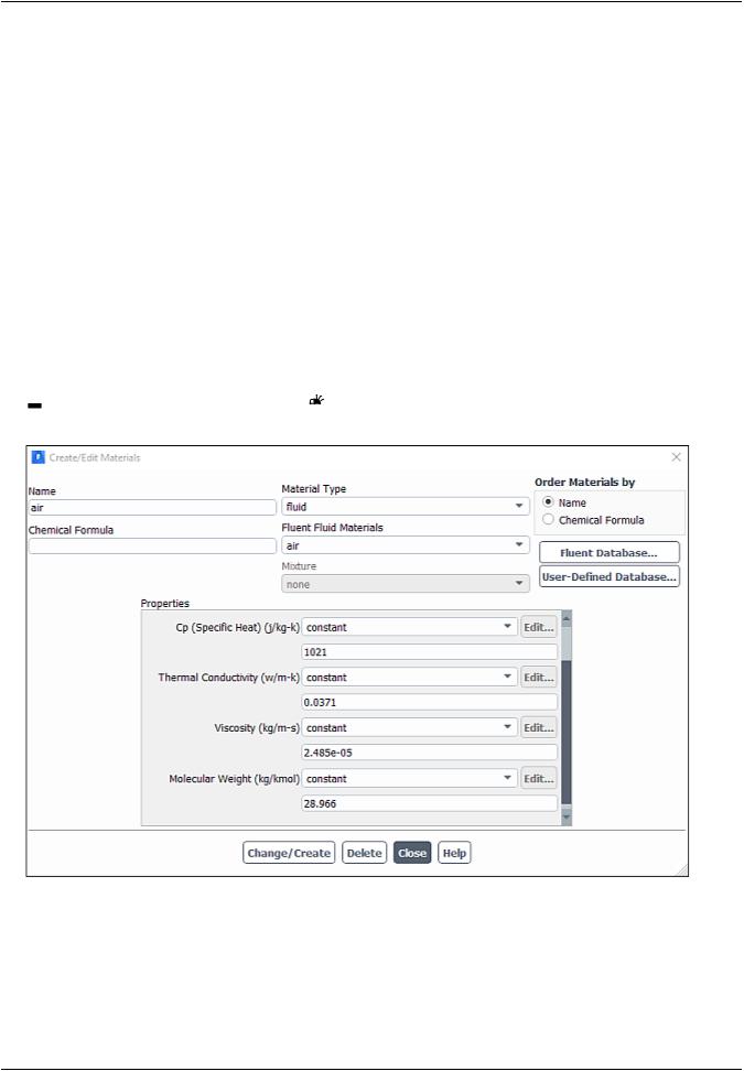
1. Set the properties for air.

Setup → Materials → Fluids → air Edit...

a.Select ideal-gas from the Density drop-down list.

b.Enter 1021 J/kg-K for Cp (Specific Heat).

c.Enter 0.0371 W/m-K for Thermal Conductivity.

d.Enter 2.485e-05 kg/m-s for Viscosity.

	Release 2019 R1 - © ANSYS,Inc.All rights reserved.- Contains proprietary and confidential information
284	of ANSYS, Inc. and its subsidiaries and affiliates.

vk.com/club152685050 | vk.com/id446425943

Setup and Solution

e.Retain the default value of 28.966 kg/kmol for Molecular Weight.

f.Click Change/Create and close the Create/Edit Materials dialog box.

2.Define the new material, insulation.

Setup → Materials → Solid → aluminum Edit...

a.Enter insulation for Name.

b.Delete the entry in the Chemical Formula field.

c.Enter 50 kg/m3 for Density.

d.Enter 800 J/kg-K for Cp (Specific Heat).

e.Enter 0.09 W/m-K for Thermal Conductivity.

f.Click Change/Create.

g.Click No when the Question dialog box appears, asking if you want to overwrite aluminum.

h.Close the Create/Edit Materials dialog box.

8.4.6. Operating Conditions

Specify operating density.

Physics → Solver → Operating Conditions...

Release 2019 R1 - © ANSYS,Inc.All rights reserved.- Contains proprietary and confidential information
of ANSYS, Inc. and its subsidiaries and affiliates.	285

vk.com/club152685050Modeling Radiation and|Naturalvk.com/id446425943Convection

1.In the Operating Conditions dialog box, select the Specified Operating Density check box.

2.Enter 0 for Operating Density and click OK to close the Operating Conditions dialog box.

8.4.7. Boundary Conditions

1. Set the boundary conditions for the front wall (w-high-x).

Setup → Boundary Conditions → w-high-x Edit...

	Release 2019 R1 - © ANSYS,Inc.All rights reserved.- Contains proprietary and confidential information
286	of ANSYS, Inc. and its subsidiaries and affiliates.

vk.com/club152685050 | vk.com/id446425943

Setup and Solution

The Wall dialog box opens.

Release 2019 R1 - © ANSYS,Inc.All rights reserved.- Contains proprietary and confidential information
of ANSYS, Inc. and its subsidiaries and affiliates.	287

vk.com/club152685050Modeling Radiation and|Naturalvk.com/id446425943Convection

a.Click the Thermal tab and select Mixed from the Thermal Conditions list.

b.Select insulation from the Material Name drop-down list.

c.Enter 5 W/m2-K for Heat Transfer Coefficient.

d.Enter 293.15 K for Free Stream Temperature.

e.Enter 0.75 for External Emissivity.

f.Enter 293.15 K for External Radiation Temperature.

g.Enter 0.95 for Internal Emissivity.

h.Enter 0.05 m for Wall Thickness.

i.Click OK to close the Wall dialog box.

2.Copy boundary conditions to define the side walls w-high-z and w-low-z.

Setup → Boundary Conditions → w-high-x Copy...

a.Ensure w-high-x is selected in the From Boundary Zone selection list.

b.Select w-high-z and w-low-z from the To Boundary Zones selection list.

c.Click Copy.

d.Click OK when the Question dialog box opens asking whether you want to copy the boundary conditions of w-high-x to all the selected zones.

e.Close the Copy Conditions dialog box.

3.Set the boundary conditions for the heated wall (w-low-x).

Setup → Boundary Conditions → w-low-x Edit...

	Release 2019 R1 - © ANSYS,Inc.All rights reserved.- Contains proprietary and confidential information
288	of ANSYS, Inc. and its subsidiaries and affiliates.

vk.com/club152685050 | vk.com/id446425943

Setup and Solution

a.Click the Thermal tab and select Temperature from the Thermal Conditions list.

b.Retain the default selection of aluminum from the Material Name drop-down list.

c.Enter 473.15 K for Temperature.

d.Enter 0.95 for Internal Emissivity.

e.Click OK to close the Wall dialog box.

4.Set the boundary conditions for the top wall (w-high-y).

Setup → Boundary Conditions → w-high-y Edit...

Release 2019 R1 - © ANSYS,Inc.All rights reserved.- Contains proprietary and confidential information
of ANSYS, Inc. and its subsidiaries and affiliates.	289

vk.com/club152685050Modeling Radiation and|Naturalvk.com/id446425943Convection

a.Click the Thermal tab and select Mixed from the Thermal Conditions list.

b.Select insulation from the Material Name drop-down list.

c.Enter 3 W/m2-K for Heat Transfer Coefficient.

d.Enter 293.15 K for Free Stream Temperature.

e.Enter 0.75 for External Emissivity.

f.Enter 293.15 K for External Radiation Temperature.

g.Enter 0.95 for Internal Emissivity.

h.Enter 0.05 m for Wall Thickness.

i.Click OK to close the Wall dialog box.

5.Copy boundary conditions to define the bottom wall (w-low-y) as previously done in this tutorial.

Setup → Boundary Conditions → w-high-y Copy...

	Release 2019 R1 - © ANSYS,Inc.All rights reserved.- Contains proprietary and confidential information
290	of ANSYS, Inc. and its subsidiaries and affiliates.