vk.com/club152685050Fluid Flow and Heat Transfer| vk.incom/id446425943a Mixing Elbow

3. Right click in the graphics window and select Refresh Display

4.Clicking the Fit to Window icon, , will cause the object to fit exactly and be centered in the window.

5.Check the mesh.

Domain → Mesh → Check → Perform Mesh Check

Note

It is a good idea to check the mesh after you manipulate it (that is, scale, convert to polyhedra, merge, separate, fuse, add zones, or smooth and swap). This will ensure that the quality of the mesh has not been compromised.

2.4.5. Setting Up Physics

In the steps that follow, you will select a solver and specify physical models, material properties, and zone conditions for your simulation using the Physics ribbon tab.

1.In the Solver group box of the Physics ribbon tab, retain the default selection of the steady pressure-based solver.

Physics → Solver

	Release 2019 R1 - © ANSYS,Inc.All rights reserved.- Contains proprietary and confidential information
46	of ANSYS, Inc. and its subsidiaries and affiliates.

vk.com/club152685050 | vk.com/id446425943

Setup and Solution

2. Set up your models for the CFD simulation using the Models group box of the Physics ribbon tab.

Note

You can also use the Models task page, which can be accessed from the tree by expanding Setup and double-clicking the Models tree item.

a.Enable heat transfer by activating the energy equation.

In the Physics ribbon tab, enable Energy (Models group box).

Physics → Models → Energy

Note

You can also double-click the Setup/Models/Energy tree item and enable the energy equation in the Energy dialog box.

b.Enable the - turbulence model.

Physics → Models → Viscous...

Release 2019 R1 - © ANSYS,Inc.All rights reserved.- Contains proprietary and confidential information
of ANSYS, Inc. and its subsidiaries and affiliates.	47

vk.com/club152685050Fluid Flow and Heat Transfer| vk.incom/id446425943a Mixing Elbow

i.Select k-epsilon from the Model list.

The Viscous Model dialog box will expand.

	Release 2019 R1 - © ANSYS,Inc.All rights reserved.- Contains proprietary and confidential information
48	of ANSYS, Inc. and its subsidiaries and affiliates.

vk.com/club152685050 | vk.com/id446425943

Setup and Solution

ii.Retain the default selection of Standard in the k-epsilon Model group box.

iii.Select Enhanced Wall Treatment in the Near-Wall Treatment group box.

Note

The default Standard Wall Functions are generally applicable if the first cell center adjacent to the wall has a y+ larger than 30. In contrast, the Enhanced Wall Treatment option provides consistent solutions for all y+ values. Enhanced Wall Treatment is recommended when using the k-epsilon model for general singlephase fluid flow problems. For more information about Near Wall Treatments in the k-epsilon model, refer to the Fluent User's Guide.

iv.Click OK to accept all the other default settings and close the Viscous Model dialog box.

Note that the Viscous... label in the ribbon is displayed in blue to indicate that the Viscous model is enabled. Also Energy and Viscous appear as enabled under the Setup/Models tree branch.

Note

While the ribbon is the primary tool for setting up and solving your problem, the tree is a dynamic representation of your case. The models, materials, conditions, and other settings that you have specified in your problem will appear in the tree. Many of the frequently used ribbon items are also available via the right-click functionality of the tree.

3. Set up the materials for the CFD simulation using the Materials group box of the Physics ribbon tab.

Create a new material called water using the Create/Edit Materials dialog box.

a.In the Physics ribbon tab, click Create/Edit... (Materials group box).

Physics → Materials → Create/Edit...

Release 2019 R1 - © ANSYS,Inc.All rights reserved.- Contains proprietary and confidential information
of ANSYS, Inc. and its subsidiaries and affiliates.	49

vk.com/club152685050Fluid Flow and Heat Transfer| vk.incom/id446425943a Mixing Elbow

b.Copy the material water-liquid (h2o < l >) from the materials database (accessed by clicking the Fluent Database... button).

c.Select water-liquid (h2o < l >) from the materials list and Click Copy, then close the Fluent Database...

panel.

	Release 2019 R1 - © ANSYS,Inc.All rights reserved.- Contains proprietary and confidential information
50	of ANSYS, Inc. and its subsidiaries and affiliates.

vk.com/club152685050 | vk.com/id446425943

Setup and Solution

d.Ensure that there are now two materials (water-liquid and air) defined locally by examining the Fluent Fluid Materials drop-down list.

Both the materials will also be listed under Fluid in the Materials task page and under the Materials tree branch.

e.Close the Create/Edit Materials dialog box.

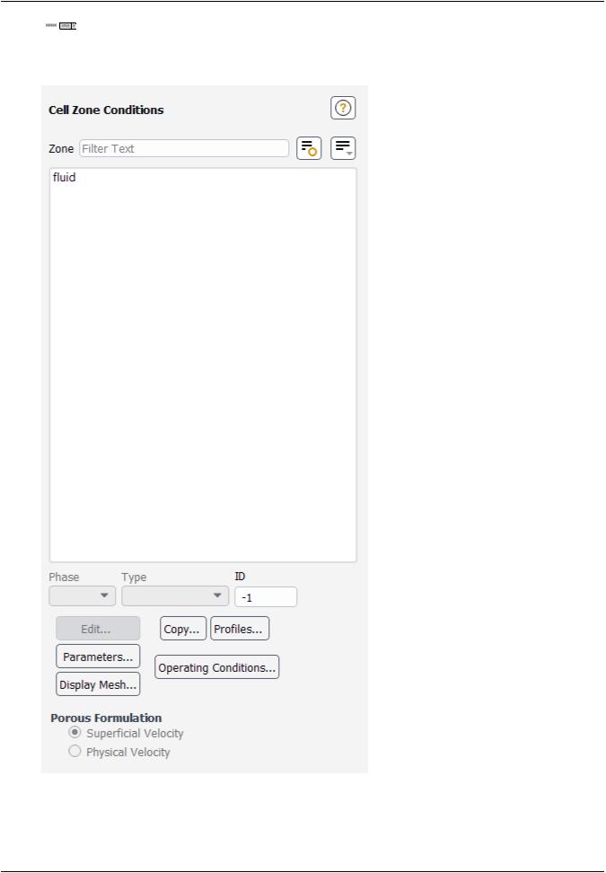
4.Set up the cell zone conditions for the fluid zone (fluid) using the Zones group box of the Physics ribbon tab.

a. In the Physics tab, click Cell Zones (Zones group box).

Release 2019 R1 - © ANSYS,Inc.All rights reserved.- Contains proprietary and confidential information
of ANSYS, Inc. and its subsidiaries and affiliates.	51

vk.com/club152685050Fluid Flow and Heat Transfer| vk.incom/id446425943a Mixing Elbow

Physics → Zones → Cell Zones

This opens the Cell Zone Conditions task page.

b. Double-click fluid in the Zone list to open the Fluid dialog box.

	Release 2019 R1 - © ANSYS,Inc.All rights reserved.- Contains proprietary and confidential information
52	of ANSYS, Inc. and its subsidiaries and affiliates.

vk.com/club152685050 | vk.com/id446425943

Setup and Solution

Note

You can also double-click the Setup/Cell Zone Conditions/fluid tree item in order to open the corresponding dialog box.

c.Select water-liquid from the Material Name drop-down list.

d.Click OK to close the Fluid dialog box.

5.Set up the boundary conditions for the inlets, outlet, and walls for your CFD analysis using the Zones group box of the Physics ribbon tab.

a.In the Physics tab, click Boundaries (Zones group box).

Physics → Zones → Boundaries

This opens the Boundary Conditions task page where the boundaries defined in your simulation are displayed in the Zone selection list.

Release 2019 R1 - © ANSYS,Inc.All rights reserved.- Contains proprietary and confidential information
of ANSYS, Inc. and its subsidiaries and affiliates.	53

vk.com/club152685050Fluid Flow and Heat Transfer| vk.incom/id446425943a Mixing Elbow

Note

To display boundary zones grouped by zone type (as shown previously), click the

Toggle Tree View button () in the upper right corner of the Boundary Conditions task page and select Zone Type under Group By.

	Release 2019 R1 - © ANSYS,Inc.All rights reserved.- Contains proprietary and confidential information
54	of ANSYS, Inc. and its subsidiaries and affiliates.

vk.com/club152685050 | vk.com/id446425943

Setup and Solution

Here the zones have names with numerical identifying tags. It is good practice to give boundaries meaningful names in a meshing application to help when you set up the model. You can also change boundary names in Fluent by simply editing the boundary and making revisions in the

Zone Name text box.

b. Set the boundary conditions at the cold inlet (velocity-inlet-5).

Tip

If you are unsure of which inlet zone corresponds to the cold inlet, you can probe

the mesh display using the right mouse button or the probe toolbar button () as described previously in this tutorial. The information will be displayed in the ANSYS Fluent console, and the zone you probed will be automatically selected from the Zone selection list in the Boundary Conditions task page.

i.Double-click velocity-inlet-5 to open the Velocity Inlet dialog box.

ii.Retain the default selection of Magnitude, Normal to Boundary from the Velocity Specification Method drop-down list.

iii.Enter 0.4 [m/s] for Velocity Magnitude.

iv.In the Turbulence group box, select Intensity and Hydraulic Diameter from the Specification Method drop-down list.

v.Retain the default value of 5 [%] for Turbulent Intensity.

Release 2019 R1 - © ANSYS,Inc.All rights reserved.- Contains proprietary and confidential information
of ANSYS, Inc. and its subsidiaries and affiliates.	55

vk.com/club152685050Fluid Flow and Heat Transfer| vk.incom/id446425943a Mixing Elbow

vi.Enter 4 [inches] for Hydraulic Diameter.

The hydraulic diameter is defined as:

where is the cross-sectional area and is the wetted perimeter.

vii.Click the Thermal tab.

viii.Enter 293.15 [K] for Temperature.

ix.Click OK to close the Velocity Inlet dialog box.

Note

You can also access the Velocity Inlet dialog box by double-clicking the

Setup/Boundary Conditions/velocity-inlet-5 tree item.

c.In a similar manner, set the boundary conditions at the hot inlet (velocity-inlet-6), using the values in the following table:

Setting	Value
Velocity Specification Method	Magnitude, Normal to Boundary

	Release 2019 R1 - © ANSYS,Inc.All rights reserved.- Contains proprietary and confidential information
56	of ANSYS, Inc. and its subsidiaries and affiliates.

vk.com/club152685050 | vk.com/id446425943		Setup and Solution
Setting		Value
Velocity Magnitude	1.2 [m/s]
Specification Method	Intensity and Hydraulic Diameter
Turbulent Intensity	5	[%]
Hydraulic Diameter	1	[inch]
Temperature	313.15 [K]

d.Double-click pressure-outlet-7 in the Zone selection list and set the boundary conditions at the outlet, as shown in the following figure.

Note

•You do not need to set a backflow temperature in this case (in the Thermal tab) because the material properties are not functions of temperature. If they were, a flow-weighted average of the inlet conditions would be a good starting value.

•ANSYS Fluent will use the backflow conditions only if the fluid is flowing into the computational domain through the outlet. Since backflow might occur at some point during the

Release 2019 R1 - © ANSYS,Inc.All rights reserved.- Contains proprietary and confidential information
of ANSYS, Inc. and its subsidiaries and affiliates.	57