vk.com/club152685050 | vk.com/id446425943	Setup and Solution
Name	force-lift
Wall Zones	wall
X-Component	0
Y-Component	1

Tip

If the Name field is not available in the Create New Observable dialog box, select a different observable type and then select force again to make it available.

When you have configured the force-lift observable, click OK to commit the settings for force-lift and close the Manage Adjoint Observables dialog box.

24.4.3. Step 3: Compute the Drag Sensitivity

1.In the Adjoint Observables dialog box (Figure 24.7: Adjoint Observables Dialog Box (p. 801)) specify that you will solve for the drag sensitivity.

Figure 24.7: Adjoint Observables Dialog Box

a.Select force-drag in the list of Observable Names.

The selection in the Adjoint Obervables dialog box determines the observable for which sensitivities will be computed. You will first compute the drag sensitivities.

b.Select Minimize from the Sensitivity Orientation list, because you are trying to reduce the drag force. This indicates that postprocessed results for the drag sensitivity will be displayed such that a reduction in drag is achieved by a design change in the positive sensitivity direction.

Release 2019 R1 - © ANSYS,Inc.All rights reserved.- Contains proprietary and confidential information
of ANSYS, Inc. and its subsidiaries and affiliates.	801

vk.com/club152685050Using the Adjoint Solver|–vk2D.com/id446425943La inar Flow Past a Cylinder

c. Click Evaluate to print the value of the drag force on the wall in the console.

Observable name: force-drag

Observable Value (n) = 1271.7444

This value is in SI units, with n denoting Newtons.

2.Adjust the solution controls.

The default solution control settings are chosen to provide robust solution advancement for a wide variety of problems, including those having complex geometry, high local flow rates, and turbulence. Given sufficient iterations, a converged result can often be obtained without modifying the controls.

For this simple laminar flow case, more aggressive settings will yield faster convergence.

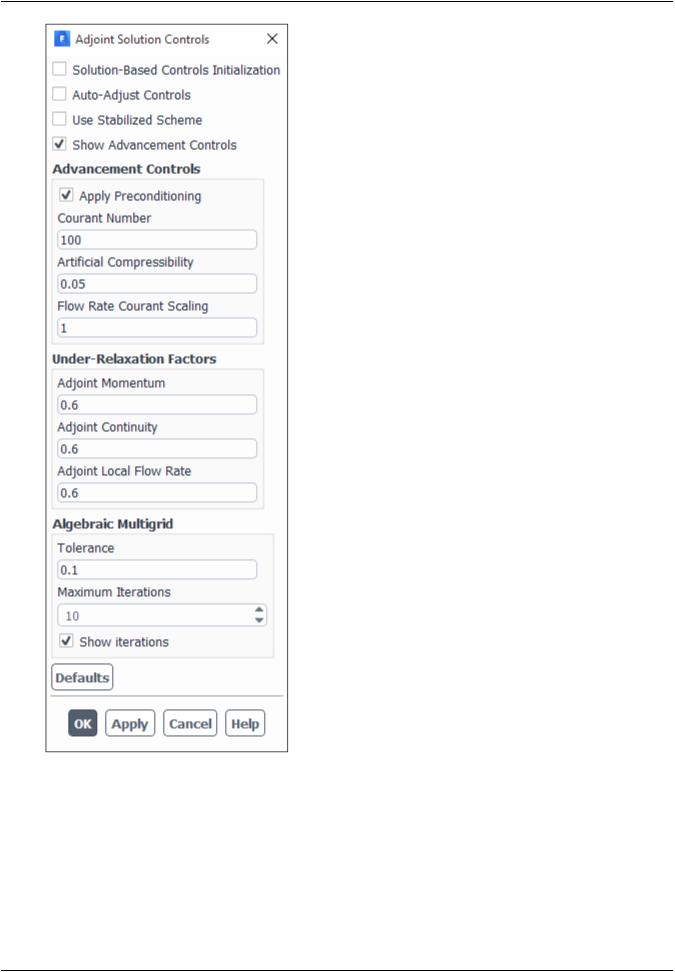
Open the Adjoint Solution Controls dialog box (Figure 24.8: Adjoint Solution Controls Dialog Box (p. 802)).

Design → Adjoint-Based → Solver Controls...

Figure 24.8: Adjoint Solution Controls Dialog Box

a.Disable the Solution-Based Controls Initialization and Auto-Adjust Controls options.

This prevents Fluent from automatically choosing and adjusting the solution controls for you.

b.Enable Show Advancement Controls.

	Release 2019 R1 - © ANSYS,Inc.All rights reserved.- Contains proprietary and confidential information
802	of ANSYS, Inc. and its subsidiaries and affiliates.

vk.com/club152685050 | vk.com/id446425943

Setup and Solution

c.Ensure that the Apply Preconditioning option is enabled. Preconditioning can help the calculation progress in a stable manner.

d.Enter 100 for Courant Number.

Higher Courant Number values correspond to more aggressive settings / faster convergence, which is appropriate for a simple case such as this.

e.Enter 0.05 for Artificial Compressibility.

Release 2019 R1 - © ANSYS,Inc.All rights reserved.- Contains proprietary and confidential information
of ANSYS, Inc. and its subsidiaries and affiliates.	803

vk.com/club152685050Using the Adjoint Solver|–vk2D.com/id446425943La inar Flow Past a Cylinder

f. Click OK to close the dialog box.

3.Configure the adjoint solution monitors by opening the Adjoint Residual Monitors dialog box (Figure 24.9: Adjoint Residual Monitors Dialog Box (p. 804)).

Design → Adjoint-Based → Monitors...

Figure 24.9: Adjoint Residual Monitors Dialog Box

In the Adjoint Residual Monitors dialog box, you set the adjoint equations that will be checked for convergence, as well as set the corresponding convergence criteria.

a.Make sure that the Print to Console and Plot options are enabled.

b.Keep the default values of 1e-05 for Adjoint continuity and Adjoint velocity, and 0.001 for Adjoint local flow rate. These settings are adequate for most cases. Make sure that the Check Convergence options are enabled.

c.Click OK to close the dialog box.

4.Run the adjoint solver using the Run Adjoint Calculation dialog box (Figure 24.10: Run Adjoint Calculation Dialog Box (p. 805)).

Design → Adjoint-Based → Calculate...

	Release 2019 R1 - © ANSYS,Inc.All rights reserved.- Contains proprietary and confidential information
804	of ANSYS, Inc. and its subsidiaries and affiliates.