

- •ANSYS Fluent Tutorial Guide
- •Table of Contents
- •Using This Manual
- •1. What’s In This Manual
- •2. How To Use This Manual
- •2.1. For the Beginner
- •2.2. For the Experienced User
- •3. Typographical Conventions Used In This Manual
- •Chapter 1: Fluid Flow in an Exhaust Manifold
- •1.1. Introduction
- •1.2. Prerequisites
- •1.3. Problem Description
- •1.4. Setup and Solution
- •1.4.1. Preparation
- •1.4.2. Meshing Workflow
- •1.4.3. General Settings
- •1.4.4. Solver Settings
- •1.4.5. Models
- •1.4.6. Materials
- •1.4.7. Cell Zone Conditions
- •1.4.8. Boundary Conditions
- •1.4.9. Solution
- •1.4.10. Postprocessing
- •1.5. Summary
- •Chapter 2: Fluid Flow and Heat Transfer in a Mixing Elbow
- •2.1. Introduction
- •2.2. Prerequisites
- •2.3. Problem Description
- •2.4. Setup and Solution
- •2.4.1. Preparation
- •2.4.2. Launching ANSYS Fluent
- •2.4.3. Reading the Mesh
- •2.4.4. Setting Up Domain
- •2.4.5. Setting Up Physics
- •2.4.6. Solving
- •2.4.7. Displaying the Preliminary Solution
- •2.4.8. Adapting the Mesh
- •2.5. Summary
- •Chapter 3: Postprocessing
- •3.1. Introduction
- •3.2. Prerequisites
- •3.3. Problem Description
- •3.4. Setup and Solution
- •3.4.1. Preparation
- •3.4.2. Reading the Mesh
- •3.4.3. Manipulating the Mesh in the Viewer
- •3.4.4. Adding Lights
- •3.4.5. Creating Isosurfaces
- •3.4.6. Generating Contours
- •3.4.7. Generating Velocity Vectors
- •3.4.8. Creating an Animation
- •3.4.9. Displaying Pathlines
- •3.4.10. Creating a Scene With Vectors and Contours
- •3.4.11. Advanced Overlay of Pathlines on a Scene
- •3.4.12. Creating Exploded Views
- •3.4.13. Animating the Display of Results in Successive Streamwise Planes
- •3.4.14. Generating XY Plots
- •3.4.15. Creating Annotation
- •3.4.16. Saving Picture Files
- •3.4.17. Generating Volume Integral Reports
- •3.5. Summary
- •Chapter 4: Modeling Periodic Flow and Heat Transfer
- •4.1. Introduction
- •4.2. Prerequisites
- •4.3. Problem Description
- •4.4. Setup and Solution
- •4.4.1. Preparation
- •4.4.2. Mesh
- •4.4.3. General Settings
- •4.4.4. Models
- •4.4.5. Materials
- •4.4.6. Cell Zone Conditions
- •4.4.7. Periodic Conditions
- •4.4.8. Boundary Conditions
- •4.4.9. Solution
- •4.4.10. Postprocessing
- •4.5. Summary
- •4.6. Further Improvements
- •Chapter 5: Modeling External Compressible Flow
- •5.1. Introduction
- •5.2. Prerequisites
- •5.3. Problem Description
- •5.4. Setup and Solution
- •5.4.1. Preparation
- •5.4.2. Mesh
- •5.4.3. Solver
- •5.4.4. Models
- •5.4.5. Materials
- •5.4.6. Boundary Conditions
- •5.4.7. Operating Conditions
- •5.4.8. Solution
- •5.4.9. Postprocessing
- •5.5. Summary
- •5.6. Further Improvements
- •Chapter 6: Modeling Transient Compressible Flow
- •6.1. Introduction
- •6.2. Prerequisites
- •6.3. Problem Description
- •6.4. Setup and Solution
- •6.4.1. Preparation
- •6.4.2. Reading and Checking the Mesh
- •6.4.3. Solver and Analysis Type
- •6.4.4. Models
- •6.4.5. Materials
- •6.4.6. Operating Conditions
- •6.4.7. Boundary Conditions
- •6.4.8. Solution: Steady Flow
- •6.4.9. Enabling Time Dependence and Setting Transient Conditions
- •6.4.10. Specifying Solution Parameters for Transient Flow and Solving
- •6.4.11. Saving and Postprocessing Time-Dependent Data Sets
- •6.5. Summary
- •6.6. Further Improvements
- •Chapter 7: Modeling Flow Through Porous Media
- •7.1. Introduction
- •7.2. Prerequisites
- •7.3. Problem Description
- •7.4. Setup and Solution
- •7.4.1. Preparation
- •7.4.2. Mesh
- •7.4.3. General Settings
- •7.4.4. Models
- •7.4.5. Materials
- •7.4.6. Cell Zone Conditions
- •7.4.7. Boundary Conditions
- •7.4.8. Solution
- •7.4.9. Postprocessing
- •7.5. Summary
- •7.6. Further Improvements
- •Chapter 8: Modeling Radiation and Natural Convection
- •8.1. Introduction
- •8.2. Prerequisites
- •8.3. Problem Description
- •8.4. Setup and Solution
- •8.4.1. Preparation
- •8.4.2. Reading and Checking the Mesh
- •8.4.3. Solver and Analysis Type
- •8.4.4. Models
- •8.4.5. Defining the Materials
- •8.4.6. Operating Conditions
- •8.4.7. Boundary Conditions
- •8.4.8. Obtaining the Solution
- •8.4.9. Postprocessing
- •8.4.10. Comparing the Contour Plots after Varying Radiating Surfaces
- •8.4.11. S2S Definition, Solution, and Postprocessing with Partial Enclosure
- •8.5. Summary
- •8.6. Further Improvements
- •Chapter 9: Using a Single Rotating Reference Frame
- •9.1. Introduction
- •9.2. Prerequisites
- •9.3. Problem Description
- •9.4. Setup and Solution
- •9.4.1. Preparation
- •9.4.2. Mesh
- •9.4.3. General Settings
- •9.4.4. Models
- •9.4.5. Materials
- •9.4.6. Cell Zone Conditions
- •9.4.7. Boundary Conditions
- •9.4.8. Solution Using the Standard k- ε Model
- •9.4.9. Postprocessing for the Standard k- ε Solution
- •9.4.10. Solution Using the RNG k- ε Model
- •9.4.11. Postprocessing for the RNG k- ε Solution
- •9.5. Summary
- •9.6. Further Improvements
- •9.7. References
- •Chapter 10: Using Multiple Reference Frames
- •10.1. Introduction
- •10.2. Prerequisites
- •10.3. Problem Description
- •10.4. Setup and Solution
- •10.4.1. Preparation
- •10.4.2. Mesh
- •10.4.3. Models
- •10.4.4. Materials
- •10.4.5. Cell Zone Conditions
- •10.4.6. Boundary Conditions
- •10.4.7. Solution
- •10.4.8. Postprocessing
- •10.5. Summary
- •10.6. Further Improvements
- •Chapter 11: Using Sliding Meshes
- •11.1. Introduction
- •11.2. Prerequisites
- •11.3. Problem Description
- •11.4. Setup and Solution
- •11.4.1. Preparation
- •11.4.2. Mesh
- •11.4.3. General Settings
- •11.4.4. Models
- •11.4.5. Materials
- •11.4.6. Cell Zone Conditions
- •11.4.7. Boundary Conditions
- •11.4.8. Operating Conditions
- •11.4.9. Mesh Interfaces
- •11.4.10. Solution
- •11.4.11. Postprocessing
- •11.5. Summary
- •11.6. Further Improvements
- •Chapter 12: Using Overset and Dynamic Meshes
- •12.1. Prerequisites
- •12.2. Problem Description
- •12.3. Preparation
- •12.4. Mesh
- •12.5. Overset Interface Creation
- •12.6. Steady-State Case Setup
- •12.6.1. General Settings
- •12.6.2. Models
- •12.6.3. Materials
- •12.6.4. Operating Conditions
- •12.6.5. Boundary Conditions
- •12.6.6. Reference Values
- •12.6.7. Solution
- •12.7. Unsteady Setup
- •12.7.1. General Settings
- •12.7.2. Compile the UDF
- •12.7.3. Dynamic Mesh Settings
- •12.7.4. Report Generation for Unsteady Case
- •12.7.5. Run Calculations for Unsteady Case
- •12.7.6. Overset Solution Checking
- •12.7.7. Postprocessing
- •12.7.8. Diagnosing an Overset Case
- •12.8. Summary
- •Chapter 13: Modeling Species Transport and Gaseous Combustion
- •13.1. Introduction
- •13.2. Prerequisites
- •13.3. Problem Description
- •13.4. Background
- •13.5. Setup and Solution
- •13.5.1. Preparation
- •13.5.2. Mesh
- •13.5.3. General Settings
- •13.5.4. Models
- •13.5.5. Materials
- •13.5.6. Boundary Conditions
- •13.5.7. Initial Reaction Solution
- •13.5.8. Postprocessing
- •13.5.9. NOx Prediction
- •13.6. Summary
- •13.7. Further Improvements
- •Chapter 14: Using the Eddy Dissipation and Steady Diffusion Flamelet Combustion Models
- •14.1. Introduction
- •14.2. Prerequisites
- •14.3. Problem Description
- •14.4. Setup and Solution
- •14.4.1. Preparation
- •14.4.2. Mesh
- •14.4.3. Solver Settings
- •14.4.4. Models
- •14.4.5. Boundary Conditions
- •14.4.6. Solution
- •14.4.7. Postprocessing for the Eddy-Dissipation Solution
- •14.5. Steady Diffusion Flamelet Model Setup and Solution
- •14.5.1. Models
- •14.5.2. Boundary Conditions
- •14.5.3. Solution
- •14.5.4. Postprocessing for the Steady Diffusion Flamelet Solution
- •14.6. Summary
- •Chapter 15: Modeling Surface Chemistry
- •15.1. Introduction
- •15.2. Prerequisites
- •15.3. Problem Description
- •15.4. Setup and Solution
- •15.4.1. Preparation
- •15.4.2. Reading and Checking the Mesh
- •15.4.3. Solver and Analysis Type
- •15.4.4. Specifying the Models
- •15.4.5. Defining Materials and Properties
- •15.4.6. Specifying Boundary Conditions
- •15.4.7. Setting the Operating Conditions
- •15.4.8. Simulating Non-Reacting Flow
- •15.4.9. Simulating Reacting Flow
- •15.4.10. Postprocessing the Solution Results
- •15.5. Summary
- •15.6. Further Improvements
- •Chapter 16: Modeling Evaporating Liquid Spray
- •16.1. Introduction
- •16.2. Prerequisites
- •16.3. Problem Description
- •16.4. Setup and Solution
- •16.4.1. Preparation
- •16.4.2. Mesh
- •16.4.3. Solver
- •16.4.4. Models
- •16.4.5. Materials
- •16.4.6. Boundary Conditions
- •16.4.7. Initial Solution Without Droplets
- •16.4.8. Creating a Spray Injection
- •16.4.9. Solution
- •16.4.10. Postprocessing
- •16.5. Summary
- •16.6. Further Improvements
- •Chapter 17: Using the VOF Model
- •17.1. Introduction
- •17.2. Prerequisites
- •17.3. Problem Description
- •17.4. Setup and Solution
- •17.4.1. Preparation
- •17.4.2. Reading and Manipulating the Mesh
- •17.4.3. General Settings
- •17.4.4. Models
- •17.4.5. Materials
- •17.4.6. Phases
- •17.4.7. Operating Conditions
- •17.4.8. User-Defined Function (UDF)
- •17.4.9. Boundary Conditions
- •17.4.10. Solution
- •17.4.11. Postprocessing
- •17.5. Summary
- •17.6. Further Improvements
- •Chapter 18: Modeling Cavitation
- •18.1. Introduction
- •18.2. Prerequisites
- •18.3. Problem Description
- •18.4. Setup and Solution
- •18.4.1. Preparation
- •18.4.2. Reading and Checking the Mesh
- •18.4.3. Solver Settings
- •18.4.4. Models
- •18.4.5. Materials
- •18.4.6. Phases
- •18.4.7. Boundary Conditions
- •18.4.8. Operating Conditions
- •18.4.9. Solution
- •18.4.10. Postprocessing
- •18.5. Summary
- •18.6. Further Improvements
- •Chapter 19: Using the Multiphase Models
- •19.1. Introduction
- •19.2. Prerequisites
- •19.3. Problem Description
- •19.4. Setup and Solution
- •19.4.1. Preparation
- •19.4.2. Mesh
- •19.4.3. Solver Settings
- •19.4.4. Models
- •19.4.5. Materials
- •19.4.6. Phases
- •19.4.7. Cell Zone Conditions
- •19.4.8. Boundary Conditions
- •19.4.9. Solution
- •19.4.10. Postprocessing
- •19.5. Summary
- •Chapter 20: Modeling Solidification
- •20.1. Introduction
- •20.2. Prerequisites
- •20.3. Problem Description
- •20.4. Setup and Solution
- •20.4.1. Preparation
- •20.4.2. Reading and Checking the Mesh
- •20.4.3. Specifying Solver and Analysis Type
- •20.4.4. Specifying the Models
- •20.4.5. Defining Materials
- •20.4.6. Setting the Cell Zone Conditions
- •20.4.7. Setting the Boundary Conditions
- •20.4.8. Solution: Steady Conduction
- •20.5. Summary
- •20.6. Further Improvements
- •Chapter 21: Using the Eulerian Granular Multiphase Model with Heat Transfer
- •21.1. Introduction
- •21.2. Prerequisites
- •21.3. Problem Description
- •21.4. Setup and Solution
- •21.4.1. Preparation
- •21.4.2. Mesh
- •21.4.3. Solver Settings
- •21.4.4. Models
- •21.4.6. Materials
- •21.4.7. Phases
- •21.4.8. Boundary Conditions
- •21.4.9. Solution
- •21.4.10. Postprocessing
- •21.5. Summary
- •21.6. Further Improvements
- •21.7. References
- •22.1. Introduction
- •22.2. Prerequisites
- •22.3. Problem Description
- •22.4. Setup and Solution
- •22.4.1. Preparation
- •22.4.2. Structural Model
- •22.4.3. Materials
- •22.4.4. Cell Zone Conditions
- •22.4.5. Boundary Conditions
- •22.4.6. Solution
- •22.4.7. Postprocessing
- •22.5. Summary
- •23.1. Introduction
- •23.2. Prerequisites
- •23.3. Problem Description
- •23.4. Setup and Solution
- •23.4.1. Preparation
- •23.4.2. Solver and Analysis Type
- •23.4.3. Structural Model
- •23.4.4. Materials
- •23.4.5. Cell Zone Conditions
- •23.4.6. Boundary Conditions
- •23.4.7. Dynamic Mesh Zones
- •23.4.8. Solution Animations
- •23.4.9. Solution
- •23.4.10. Postprocessing
- •23.5. Summary
- •Chapter 24: Using the Adjoint Solver – 2D Laminar Flow Past a Cylinder
- •24.1. Introduction
- •24.2. Prerequisites
- •24.3. Problem Description
- •24.4. Setup and Solution
- •24.4.1. Step 1: Preparation
- •24.4.2. Step 2: Define Observables
- •24.4.3. Step 3: Compute the Drag Sensitivity
- •24.4.4. Step 4: Postprocess and Export Drag Sensitivity
- •24.4.4.1. Boundary Condition Sensitivity
- •24.4.4.2. Momentum Source Sensitivity
- •24.4.4.3. Shape Sensitivity
- •24.4.4.4. Exporting Drag Sensitivity Data
- •24.4.5. Step 5: Compute Lift Sensitivity
- •24.4.6. Step 6: Modify the Shape
- •24.5. Summary
- •25.1. Introduction
- •25.2. Prerequisites
- •25.3. Problem Description
- •25.4. Setup and Solution
- •25.4.1. Preparation
- •25.4.2. Reading and Scaling the Mesh
- •25.4.3. Loading the MSMD battery Add-on
- •25.4.4. NTGK Battery Model Setup
- •25.4.4.1. Specifying Solver and Models
- •25.4.4.2. Defining New Materials for Cell and Tabs
- •25.4.4.3. Defining Cell Zone Conditions
- •25.4.4.4. Defining Boundary Conditions
- •25.4.4.5. Specifying Solution Settings
- •25.4.4.6. Obtaining Solution
- •25.4.5. Postprocessing
- •25.4.6. Simulating the Battery Pulse Discharge Using the ECM Model
- •25.4.7. Using the Reduced Order Method (ROM)
- •25.4.8. External and Internal Short-Circuit Treatment
- •25.4.8.1. Setting up and Solving a Short-Circuit Problem
- •25.4.8.2. Postprocessing
- •25.5. Summary
- •25.6. Appendix
- •25.7. References
- •26.1. Introduction
- •26.2. Prerequisites
- •26.3. Problem Description
- •26.4. Setup and Solution
- •26.4.1. Preparation
- •26.4.2. Reading and Scaling the Mesh
- •26.4.3. Loading the MSMD battery Add-on
- •26.4.4. Battery Model Setup
- •26.4.4.1. Specifying Solver and Models
- •26.4.4.2. Defining New Materials
- •26.4.4.3. Defining Cell Zone Conditions
- •26.4.4.4. Defining Boundary Conditions
- •26.4.4.5. Specifying Solution Settings
- •26.4.4.6. Obtaining Solution
- •26.4.5. Postprocessing
- •26.5. Summary
- •Chapter 27: In-Flight Icing Tutorial Using Fluent Icing
- •27.1. Fluent Airflow on the NACA0012 Airfoil
- •27.2. Flow Solution on the Rough NACA0012 Airfoil
- •27.3. Droplet Impingement on the NACA0012
- •27.3.1. Monodispersed Calculation
- •27.3.2. Langmuir-D Distribution
- •27.3.3. Post-Processing Using Quick-View
- •27.4. Fluent Icing Ice Accretion on the NACA0012
- •27.5. Postprocessing an Ice Accretion Solution Using CFD-Post Macros
- •27.6. Multi-Shot Ice Accretion with Automatic Mesh Displacement
- •27.7. Multi-Shot Ice Accretion with Automatic Mesh Displacement – Postprocessing Using CFD-Post

vk.com/club152685050Modeling Evaporating Liquid| vk.com/id446425943Spray
Figure 16.8: Convergence History of Total Mass in Domain
Figure 16.9: Convergence History of Evaporated Particle Mass
8. Save the case and data files (spray2.cas.gz and spray2.dat.gz).

 File → Write → Case & Data...
16.4.10. Postprocessing
1.Display the trajectories of the droplets in the spray injection (Figure 16.10: Particle Tracks for the Spray Injection (p. 588)).
This will allow you to review the location of the droplets.

 Results → Graphics → Particle Tracks → Edit...
|
Release 2019 R1 - © ANSYS,Inc.All rights reserved.- Contains proprietary and confidential information |
586 |
of ANSYS, Inc. and its subsidiaries and affiliates. |
vk.com/club152685050 | vk.com/id446425943 |
Setup and Solution |
a.Enable Draw Mesh in the Options group box.
The Mesh Display dialog box will open.
i.Retain the current display settings.
ii.Close the Mesh Display dialog box.
b.Retain the default selection of point from the Track Style drop-down list.
c.Select Particle Variables... and Particle Diameter from the Color by drop-down lists.
This will display the location of the droplets colored by their diameters.
d.Select injection-0 from the Release from Injections selection list.
e.Click Display. As an optional exercise, you can increase the particle size by clicking the Attributes... button in the Particle Tracks dialog box and adjusting the Marker Size value in the Track Style Attributes dialog box.
f.Close the Particle Tracks dialog box.
g.Restore the 30–degree section to obtain the view as shown in Figure 16.10: Particle Tracks for the Spray Injection (p. 588).
 View → Display → Views...
Release 2019 R1 - © ANSYS,Inc.All rights reserved.- Contains proprietary and confidential information |
|
of ANSYS, Inc. and its subsidiaries and affiliates. |
587 |

vk.com/club152685050Modeling Evaporating Liquid| vk.com/id446425943Spray
i.Click the Define... button to open the Graphics Periodicity dialog box.
ii.Click Reset and close the Graphics Periodicity dialog box.
iii.Close the Views dialog box.
h. Use the mouse to obtain the view shown in Figure 16.10: Particle Tracks for the Spray Injection (p. 588).
Figure 16.10: Particle Tracks for the Spray Injection
The air-blast atomizer model assumes that a cylindrical liquid sheet exits the atomizer, which then disintegrates into ligaments and droplets. Appropriately, the model determines that the droplets should be input into the domain in a ring. The radius of this disk is determined from the inner and outer radii of the injector.
Note
The maximum diameter of the droplets is about 4.9x10⁻⁵ m or 0.49 mm, which is simililar to the film height. The inner diameter and outer diameter of the injector are 3.5 mm and 4.5 mm, respectively. Hence the film height is 0.5 mm. The range in the droplet sizes is due to the fact that the air-blast atomizer automatically uses a distribution of droplet sizes.
Also note that the droplets are placed a slight distance away from the injector. Once the droplets are injected into the domain, their behavior will be determined by secondary models. For instance, they may collide/coalesce with other droplets depending on the secondary models employed. However, once a droplet has been introduced into the domain, the air-blast atomizer model no longer affects the droplet.
2.Display the mean particle temperature field (Figure 16.11: Contours of DPM Temperature (p. 590)).
 Results → Graphics → Contours → Edit...
|
Release 2019 R1 - © ANSYS,Inc.All rights reserved.- Contains proprietary and confidential information |
588 |
of ANSYS, Inc. and its subsidiaries and affiliates. |

vk.com/club152685050 | vk.com/id446425943 |
Setup and Solution |
a.Ensure that Filled is enabled in the Options group box
b.Disable Draw Mesh.
c.Select Discrete Phase Variables... and DPM Temperature from the Contours of drop-down lists.
d.Disable Auto Range.
The Clip to Range option will automatically be enabled.
e.Click Compute to update the Min and Max fields.
f.Enter 260 for Min.
g.Select angle=15 from the Surfaces selection list.
h.Click Display and close the Contours dialog box.
i.Use the mouse to obtain the view shown in Figure 16.11: Contours of DPM Temperature (p. 590).
Release 2019 R1 - © ANSYS,Inc.All rights reserved.- Contains proprietary and confidential information |
|
of ANSYS, Inc. and its subsidiaries and affiliates. |
589 |
vk.com/club152685050Modeling Evaporating Liquid| vk.com/id446425943Spray
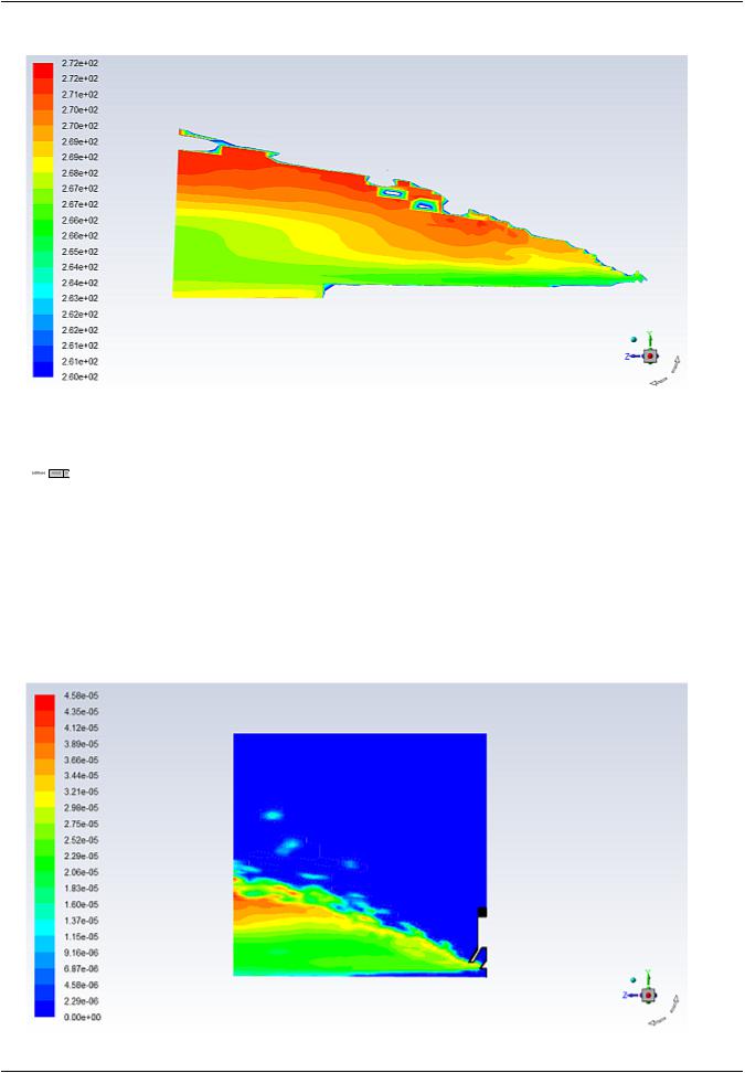
Figure 16.11: Contours of DPM Temperature
3.Display the mean Sauter diameter (Figure 16.12: Contours of DPM Sauter Diameter (p. 590)).
 Results → Graphics → Contours → Edit...
a.Enable Autorange in the Options group box.
b.Select Discrete Phase Variables... and DPM D32 from the Contours of drop-down lists.
c.Select angle=15 from the Surfaces selection list.
d.Click Display and close the Contours dialog box.
Figure 16.12: Contours of DPM Sauter Diameter
|
Release 2019 R1 - © ANSYS,Inc.All rights reserved.- Contains proprietary and confidential information |
590 |
of ANSYS, Inc. and its subsidiaries and affiliates. |

vk.com/club152685050 | vk.com/id446425943 |
Setup and Solution |
4.Display vectors of DPM mean velocity colored by DPM velocity magnitude (Figure 16.13: Vectors of DPM Mean Velocity Colored by DPM Velocity Magnitude (p. 592)).
 Results → Graphics → Vectors → Edit...
a.Select dpm-mean-velocity from the Vectors of drop-down lists.
b.Select Discrete Phase Variables... and DPM Velocity Magnitude from the Color by drop-down lists.
c.Enter 7 for Scale.
d.Select angle=15 from the Surfaces selection list.
e.Click Display and close the Contours dialog box.
Release 2019 R1 - © ANSYS,Inc.All rights reserved.- Contains proprietary and confidential information |
|
of ANSYS, Inc. and its subsidiaries and affiliates. |
591 |

vk.com/club152685050Modeling Evaporating Liquid| vk.com/id446425943Spray
Figure 16.13: Vectors of DPM Mean Velocity Colored by DPM Velocity Magnitude
5.Create an isosurface of the methanol mass fraction.

 Results → Surface → Create → Iso-Surface...
a.Enter methanol-mf=0.002 for the New Surface Name.
b.Select Species... and Mass fraction of ch3oh from the Surface of Constant drop-down lists.
c.Click Compute to update the minimum and maximum values.
d.Enter 0.002 for Iso-Values.
|
Release 2019 R1 - © ANSYS,Inc.All rights reserved.- Contains proprietary and confidential information |
592 |
of ANSYS, Inc. and its subsidiaries and affiliates. |

vk.com/club152685050 | vk.com/id446425943 |
Setup and Solution |
e.Click Create and then close the Iso-Surface dialog box.
6.Display the isosurface you just created (methanol-mf=0.002).

 Results → Graphics → Mesh → Edit...
a.Deselect atomizer-wall and select methanol-mf=0.002 in the Surfaces selection list.
b.Click the Colors... button to open the Mesh Colors dialog box.
i.Select surface in the Types list and green in the Colors list.
Scroll down the Types list to locate surface. The isosurface will now be displayed in green, which contrasts better with the rest of the mesh.
Release 2019 R1 - © ANSYS,Inc.All rights reserved.- Contains proprietary and confidential information |
|
of ANSYS, Inc. and its subsidiaries and affiliates. |
593 |

vk.com/club152685050Modeling Evaporating Liquid| vk.com/id446425943Spray
ii. Close the Mesh Colors dialog box.
c.Click Display in the Mesh Display dialog box.
The graphics display will be updated to show the isosurface.
7.Modify the view to include the entire atomizer.
 View → Display → Views...
a.Click Define... to open the Graphics Periodicity dialog box.
i.Select fluid from the Cell Zones list.
ii.Ensure that Rotational is selected from the Periodic Type list and the Number of Repeats is set to 12.
iii.Click Set and close the Graphics Periodicity dialog box.
b.Click Apply and close the Views dialog box.
c.Click Display and close the Mesh Display dialog box.
d.Use the mouse to obtain the view shown in Figure 16.14: Full Atomizer Display with Surface of Constant Methanol Mass Fraction (p. 595).
|
Release 2019 R1 - © ANSYS,Inc.All rights reserved.- Contains proprietary and confidential information |
594 |
of ANSYS, Inc. and its subsidiaries and affiliates. |

vk.com/club152685050 | vk.com/id446425943 |
Setup and Solution |
Figure 16.14: Full Atomizer Display with Surface of Constant Methanol Mass Fraction
e.This view can be improved to resemble Figure 16.15: Atomizer Display with Surface of Constant Methanol Mass Fraction Enhanced (p. 596) by changing some of the following variables:
•Disable Edges in the Mesh Display dialog box
•Select only atomizer-wall and methanol-mf=0.002 in the Surfaces list of the Mesh Display dialog box
•Change the Number of Repeats to 6 in the Graphics Periodicity dialog box
•Enable Lighting and change it to Flat in the View tab (Display group)
•Enable Headlight check in the View tab (Display group)
Release 2019 R1 - © ANSYS,Inc.All rights reserved.- Contains proprietary and confidential information |
|
of ANSYS, Inc. and its subsidiaries and affiliates. |
595 |