vk.com/club152685050 | vk.com/id446425943

Setup and Solution

d.Click the Porous Zone tab.

i.Make sure that the principal direction vectors are set as shown in Table 7.1: Values for the Principle Direction Vectors (p. 253).

ANSYS Fluent automatically calculates the third (Z direction) vector based on your inputs for the first two vectors. The direction vectors determine which axis the viscous and inertial resistance coefficients act upon.

Table 7.1: Values for the Principle Direction Vectors

Axis	Direction-1 Vector	Direction-2 Vector
X	1	0
Y	0	1
Z	0	0

ii.For the viscous and inertial resistance directions, enter the values in Table 7.2: Values for the Viscous and Inertial Resistance (p. 253) Viscous Resistance and Inertial Resistance.

Direction-2 and Direction-3 are set to arbitrary large numbers. These values are several orders

of magnitude greater than that of the Direction-1 flow and will make any radial flow insignificant. Scroll down to access the fields that are not initially visible.

Table 7.2: Values for the Viscous and Inertial Resistance
Direction	Viscous Resistance (1/m2)	Inertial Resistance (1/m)
Direction-1	3.846e+07	20.414
Direction-2	3.846e+10	20414
Direction-3	3.846e+10	20414

e. Click OK to close the Fluid dialog box.

7.4.7. Boundary Conditions

Setup → Boundary Conditions → inlet Edit...

Release 2019 R1 - © ANSYS,Inc.All rights reserved.- Contains proprietary and confidential information
of ANSYS, Inc. and its subsidiaries and affiliates.	253

vk.com/club152685050Modeling Flow Through|Porousvk.com/id446425943Media

1. Set the velocity and turbulence boundary conditions at the inlet (inlet).

	Release 2019 R1 - © ANSYS,Inc.All rights reserved.- Contains proprietary and confidential information
254	of ANSYS, Inc. and its subsidiaries and affiliates.

vk.com/club152685050 | vk.com/id446425943

Setup and Solution

a.Enter 22.6 m/s for Velocity Magnitude.

b.In the Turbulence group box, select Intensity and Hydraulic Diameter from the Specification Method drop-down list.

c.Enter 10% for the Turbulent Intensity.

d.Enter 42 mm for the Hydraulic Diameter.

e.Click OK to close the Velocity Inlet dialog box.

2.Set the boundary conditions at the outlet (outlet).

Setup → Boundary Conditions → outlet Edit...

Release 2019 R1 - © ANSYS,Inc.All rights reserved.- Contains proprietary and confidential information
of ANSYS, Inc. and its subsidiaries and affiliates.	255

vk.com/club152685050Modeling Flow Through|Porousvk.com/id446425943Media

a.Retain the default setting of 0 for Gauge Pressure.

b.In the Turbulence group box, select Intensity and Hydraulic Diameter from the Specification Method drop-down list.

c.Retain the default value of 5% for the Backflow Turbulent Intensity.

d.Enter 42 mm for the Backflow Hydraulic Diameter.

e.Click OK to close the Pressure Outlet dialog box.

3.Retain the default boundary conditions for the walls (substrate-wall and wall).

7.4.8. Solution

1.Set the solution parameters.

Solution → Solution → Methods...

	Release 2019 R1 - © ANSYS,Inc.All rights reserved.- Contains proprietary and confidential information
256	of ANSYS, Inc. and its subsidiaries and affiliates.

vk.com/club152685050 | vk.com/id446425943

Setup and Solution

Retain the default settiings.

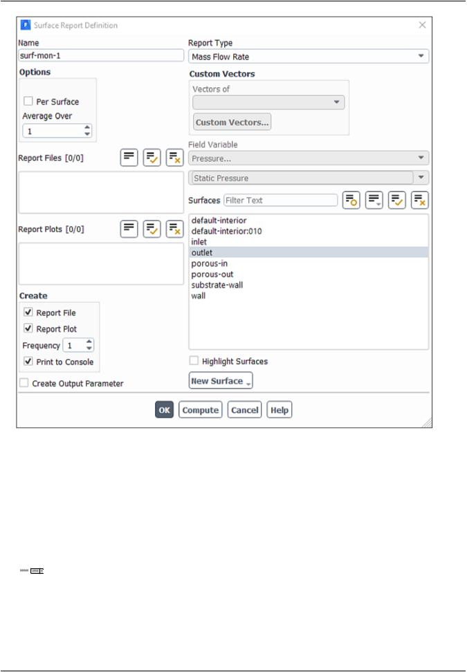
2.Enable the plotting of the mass flow rate at the outlet.

Solution → Reports → Definitions → New → Surface Report → Mass Flow Rate

Release 2019 R1 - © ANSYS,Inc.All rights reserved.- Contains proprietary and confidential information
of ANSYS, Inc. and its subsidiaries and affiliates.	257

vk.com/club152685050Modeling Flow Through|Porousvk.com/id446425943Media

a.Enter surf-mon-1 for the Name of the surface report definition.

b.In the Create group box, enable Report File, Report Plot and Print to Console.

c.Select outlet in the Surfaces selection list.

d.Click OK to save the surface report definition settings and close the Surface Report Definition dialog box.

3.Initialize the solution from the inlet.

Solution → Initialization

	Release 2019 R1 - © ANSYS,Inc.All rights reserved.- Contains proprietary and confidential information
258	of ANSYS, Inc. and its subsidiaries and affiliates.

vk.com/club152685050 | vk.com/id446425943

Setup and Solution

a. Select Standard under Method.

Warning

Standard is the recommended initialization method for porous media simulations. The default Hybrid method does not account for the porous media properties, and depending on boundary conditions, may produce an unrealistic initial velocity field. For porous media simulations, the Hybrid method should only be used when the

Maintain Constant Velocity Magnitude option is enabled in the Hybrid Initialization dialog box.

b. Click Options... to open the Solution Initialization task page, which provides access to further settings.

Release 2019 R1 - © ANSYS,Inc.All rights reserved.- Contains proprietary and confidential information
of ANSYS, Inc. and its subsidiaries and affiliates.	259

vk.com/club152685050Modeling Flow Through|Porousvk.com/id446425943Media

i.Select inlet from the Compute from drop-down list in the Solution Initialization task page.

ii.Retain the default settings for standard initialization method.

iii.Click Initialize.

4.Save the case file (catalytic_converter.cas.gz).

File → Write → Case...

5.Run the calculation by requesting 100 iterations.

Solution → Run Calculation

a. Enter 100 for No. of Iterations.

	Release 2019 R1 - © ANSYS,Inc.All rights reserved.- Contains proprietary and confidential information
260	of ANSYS, Inc. and its subsidiaries and affiliates.