vk.com/club152685050Modeling Radiation and|Naturalvk.com/id446425943Convection

Figure 8.1: Schematic of the Problem

8.4. Setup and Solution

The following sections describe the setup and solution steps for this tutorial:

8.4.1.Preparation

8.4.2.Reading and Checking the Mesh

8.4.3.Solver and Analysis Type

8.4.4.Models

8.4.5.Defining the Materials

8.4.6.Operating Conditions

8.4.7.Boundary Conditions

8.4.8.Obtaining the Solution

8.4.9.Postprocessing

8.4.10.Comparing the Contour Plots after Varying Radiating Surfaces

8.4.11.S2S Definition, Solution, and Postprocessing with Partial Enclosure

8.4.1. Preparation

To prepare for running this tutorial:

1.Download the radiation_natural_convection.zip file here.

2.Unzip radiation_natural_convection.zip to your working directory.

3.The mesh file rad.msh.gz can be found in the folder.

4.Use Fluent Launcher to start the 3D version of ANSYS Fluent.

5.Ensure that the Display Mesh After Reading option is enabled.

6.Enable Double Precision.

	Release 2019 R1 - © ANSYS,Inc.All rights reserved.- Contains proprietary and confidential information
278	of ANSYS, Inc. and its subsidiaries and affiliates.

vk.com/club152685050 | vk.com/id446425943

Setup and Solution

7.Ensure Serial is selected under Processing Options.

8.4.2. Reading and Checking the Mesh

1.Read the mesh file rad.msh.gz.

File → Read → Mesh...

As the mesh is read, messages will appear in the console reporting the progress of the reading and the mesh statistics. The mesh size will be reported as 64,000 cells. Once reading is complete, the mesh will be displayed in the graphics window.

Figure 8.2: Graphics Display of Mesh

2. Check the mesh.

Domain → Mesh → Check → Perform Mesh Check

ANSYS Fluent will perform various checks on the mesh and report the progress in the console. Make sure that the reported minimum volume is a positive number.

8.4.3. Solver and Analysis Type

1.Confirm the solver settings and enable gravity.

Setup → General

Release 2019 R1 - © ANSYS,Inc.All rights reserved.- Contains proprietary and confidential information
of ANSYS, Inc. and its subsidiaries and affiliates.	279

vk.com/club152685050Modeling Radiation and|Naturalvk.com/id446425943Convection

a.Retain the default settings of pressure-based steady-state solver in the Solver group box.

b.Enable the Gravity option.

c.Enter -9.81 m/s2 for Y in the Gravitational Acceleration group box.

8.4.4. Models

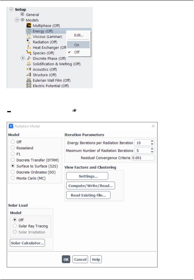
1. Enable the energy equation.

Setup → Models → Energy On

	Release 2019 R1 - © ANSYS,Inc.All rights reserved.- Contains proprietary and confidential information
280	of ANSYS, Inc. and its subsidiaries and affiliates.

vk.com/club152685050 | vk.com/id446425943

Setup and Solution

2. Set up the Surface to Surface (S2S) radiation model.

Setup → Models → Radiation Model → Surface to Surface (S2S)

Release 2019 R1 - © ANSYS,Inc.All rights reserved.- Contains proprietary and confidential information
of ANSYS, Inc. and its subsidiaries and affiliates.	281

vk.com/club152685050Modeling Radiation and|Naturalvk.com/id446425943Convection

The surface-to-surface (S2S) radiation model can be used to account for the radiation exchange in an enclosure of gray-diffuse surfaces. The energy exchange between two surfaces depends in part on their size, separation distance, and orientation. These parameters are accounted for by a geometric function called a “view factor”.

The S2S model assumes that all surfaces are gray and diffuse. Thus according to the gray-body model,

if a certain amount of radiation is incident on a surface, then a fraction is reflected, a fraction is absorbed, and a fraction is transmitted. The main assumption of the S2S model is that any absorption, emission,

or scattering of radiation by the medium can be ignored. Therefore only “surface-to-surface” radiation is considered for analysis.

For most applications the surfaces in question are opaque to thermal radiation (in the infrared spectrum), so the surfaces can be considered opaque. For gray, diffuse, and opaque surfaces it is valid to assume that the emissivity is equal to the absorptivity and that reflectivity is equal to 1 minus the emissivity.

When the S2S model is used, you also have the option to define a “partial enclosure”. This option allows you to disable the view factor calculation for walls with negligible emission/absorption or walls that have uniform temperature. The main advantage of this option is to speed up the view factor calculation and the radiosity calculation.

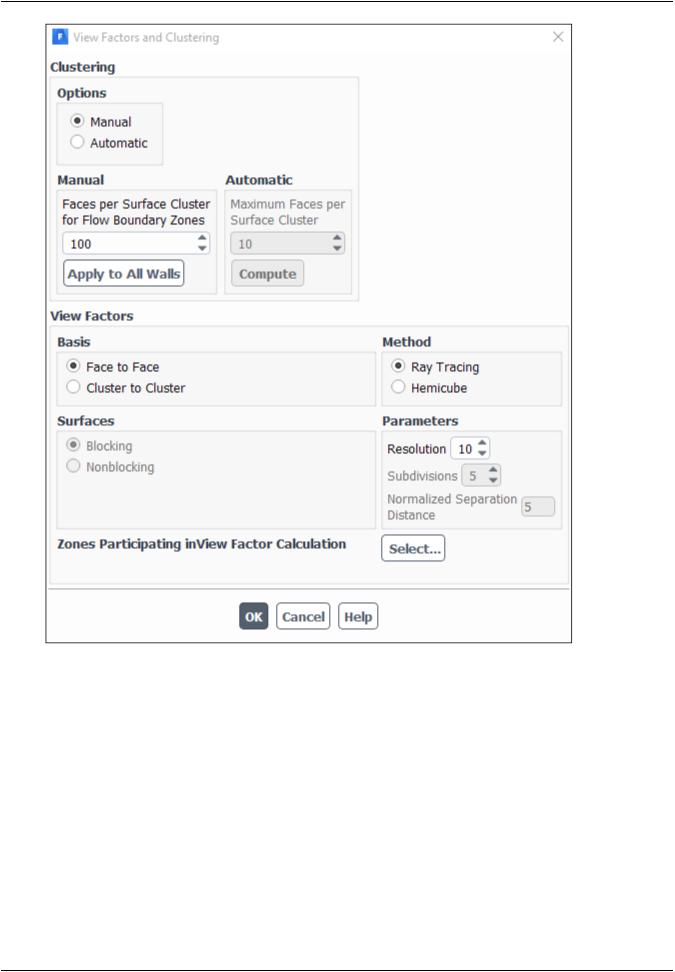
a.Click the Settings... button to open the View Factors and Clustering dialog box.

You will define the view factor and cluster parameters.

	Release 2019 R1 - © ANSYS,Inc.All rights reserved.- Contains proprietary and confidential information
282	of ANSYS, Inc. and its subsidiaries and affiliates.

vk.com/club152685050 | vk.com/id446425943

Setup and Solution

i.Enter a value of 100 for Faces per Surface Cluster for Flow Boundary Zones in the Manual group box.

ii.Click Apply to All Walls.

The S2S radiation model is computationally very expensive when there are a large number of radiating surfaces. The number of radiating surfaces is reduced by clustering surfaces into surface “clusters”. The surface clusters are made by starting from a face and adding its neighbors and their neighbors until a specified number of faces per surface cluster is collected.

For a small problem, the default value of 1 for Faces per Surface Cluster for Flow Boundary Zones is acceptable. For a large problem you can increase this number to reduce the memory requirement for the view factor file that is saved in a later step. This may also lead to some reduction in the computational expense. However, this is at the cost of some accuracy. This tutorial illustrates the influence of clusters.

iii.Ensure Ray Tracing is selected from the Method list in the View Factors group box.

Release 2019 R1 - © ANSYS,Inc.All rights reserved.- Contains proprietary and confidential information
of ANSYS, Inc. and its subsidiaries and affiliates.	283