vk.com/club152685050Using Multiple Reference| vkFrames.com/id446425943

10.4.7. Solution

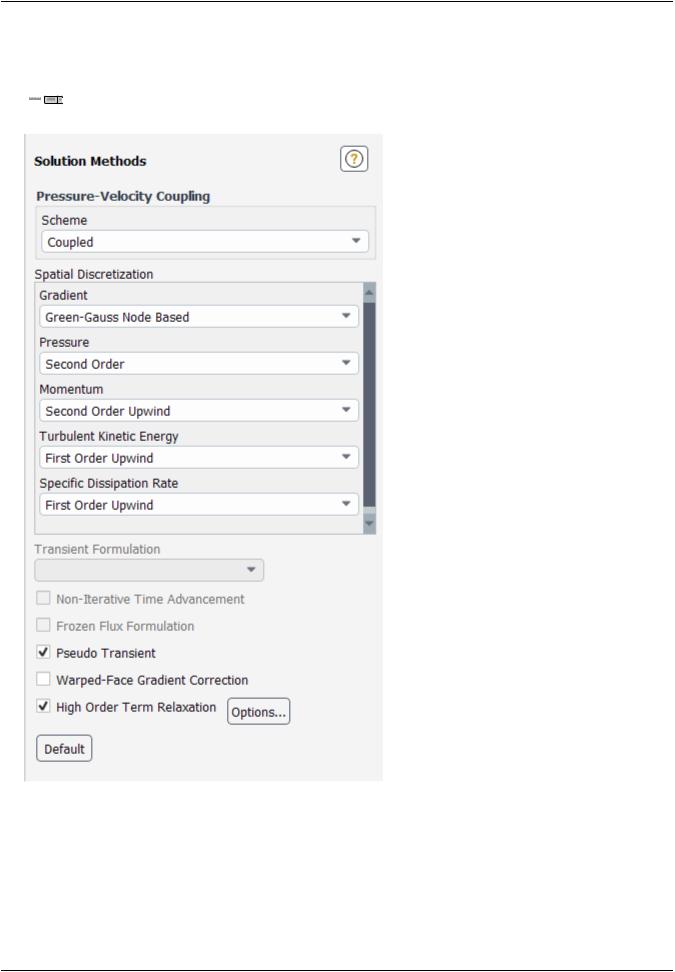
1.Specify the solution methods.

Solution → Solution → Methods...

a.Select Green-Gauss Node Based from the Gradient drop-down list in the Spatial Discretization group box.

b.Enable the High Order Term Relaxation option.

c.Retain the default selections.

2.Create a surface report definition for total pressure at the outlet.

	Release 2019 R1 - © ANSYS,Inc.All rights reserved.- Contains proprietary and confidential information
360	of ANSYS, Inc. and its subsidiaries and affiliates.

vk.com/club152685050 | vk.com/id446425943

Setup and Solution

Solution → Reports → Definitions → New → Surface Report → Mass-Weighted Average

a.Enter p-out for the Name of the surface report definition.

b.Select Pressure... and Total Pressure from the Field Variable drop-down lists.

c.Select Outlet from the Surfaces selection list.

This automatically selects all the outlet boundary conditions that have been specified.

d.Click OK to save the surface report definition settings and close the Surface Report Definition dialog box.

3.Create a surface report definition for total pressure at the inlet.

Solution → Reports → Definitions → New → Surface Report → Mass-Weighted Average

a.Enter p-in for the Name of the surface report definition.

b.Select Pressure... and Total Pressure from the Field Variable drop-down lists.

c.Select Inlet from the Surfaces selection list.

d.Click OK to save the surface report definition settings and close the Surface Report Definition dialog box.

4.Create an expression for pump head.

Solution → Reports → Definitions → New → Expression...

a. Enter the expression (p-out<rd> - p-in<rd>) / (998.2 * 9.81).

You can insert the report definitions you previously created using the Report Definitions drop-down list under Select Operand Field Functions from and clicking Select.

The expression uses 998.2 as the density of water [kg/m^3] and 9.81 as the acceleration of the fluid due to gravity [m/s^2].

b.Enter head for Name.

c.Select Report Plot

d.Select Print to Console

e.Click Define to save the expression and close the Expression Report Definition dialog box.

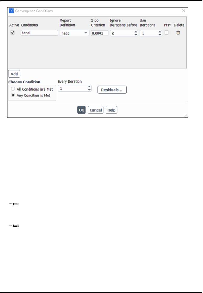
5.Specify the pump head percentage change to be the convergence condition to be used for solution monitoring.

Solution → Reports → Residuals

Release 2019 R1 - © ANSYS,Inc.All rights reserved.- Contains proprietary and confidential information
of ANSYS, Inc. and its subsidiaries and affiliates.	361

vk.com/club152685050Using Multiple Reference| vkFrames.com/id446425943

a.ClickConvergence Conditions... to add .

b.Enter head underConditions.

c.Select head underReport Defeintion.

d.Enter 0.0001 the Stop Criterion.

e.Select Any Condition is Met underChoose Condition.

f.Click OK to close the Convergence Conditions dialog box.

g.Click OK to close the Residual Monitors dialog box.

6.Save the case file (pump_volute.cas.gz).

File → Write → Case...

7.Start the calculation.

Solution → Run Calculation → Advanced...

a.Enter 5 for Timescale Factor.

b.Enter 200 for Number of Iterations.

c.Click Calculate.

d.Click Yes to initialize the case before solving.

You can monitor the progression of the residuals and the pump head during the run.

	Release 2019 R1 - © ANSYS,Inc.All rights reserved.- Contains proprietary and confidential information
362	of ANSYS, Inc. and its subsidiaries and affiliates.

vk.com/club152685050 | vk.com/id446425943

Setup and Solution

8. Save the case and data files (pump_volute.cas.gz and pump-volute.dat.gz).

File → Write → Case & Data...

10.4.8. Postprocessing

1.Determine the head generated from the pump

Solution → Reports → Definitions → Edit...

a.Select head from the Report Definitions selection list.

b.Click Compute.

The head generated by the pump is prointed to the console and is approximately, 21.5 [m].

2.Create a contour showing the flow uniformity at the outlet.

Results → Graphics → Contours → New...

a.Enable the Filled option in the Options group box.

b.Disable the Global Range option in the Options group box.

c.Select Velocity... and Velocity Magnitude from the Contours of drop-down lists.

d.Select Outlet from the Surfaces selection list.

e.Select Draw Mesh.

f.On the Mesh Display dialog box that opens, select volute-wall from the Surfaces selection list.

g.Click Display and close the Mesh Display dialog box.

Release 2019 R1 - © ANSYS,Inc.All rights reserved.- Contains proprietary and confidential information
of ANSYS, Inc. and its subsidiaries and affiliates.	363