

- •ANSYS Fluent Tutorial Guide
- •Table of Contents
- •Using This Manual
- •1. What’s In This Manual
- •2. How To Use This Manual
- •2.1. For the Beginner
- •2.2. For the Experienced User
- •3. Typographical Conventions Used In This Manual
- •Chapter 1: Fluid Flow in an Exhaust Manifold
- •1.1. Introduction
- •1.2. Prerequisites
- •1.3. Problem Description
- •1.4. Setup and Solution
- •1.4.1. Preparation
- •1.4.2. Meshing Workflow
- •1.4.3. General Settings
- •1.4.4. Solver Settings
- •1.4.5. Models
- •1.4.6. Materials
- •1.4.7. Cell Zone Conditions
- •1.4.8. Boundary Conditions
- •1.4.9. Solution
- •1.4.10. Postprocessing
- •1.5. Summary
- •Chapter 2: Fluid Flow and Heat Transfer in a Mixing Elbow
- •2.1. Introduction
- •2.2. Prerequisites
- •2.3. Problem Description
- •2.4. Setup and Solution
- •2.4.1. Preparation
- •2.4.2. Launching ANSYS Fluent
- •2.4.3. Reading the Mesh
- •2.4.4. Setting Up Domain
- •2.4.5. Setting Up Physics
- •2.4.6. Solving
- •2.4.7. Displaying the Preliminary Solution
- •2.4.8. Adapting the Mesh
- •2.5. Summary
- •Chapter 3: Postprocessing
- •3.1. Introduction
- •3.2. Prerequisites
- •3.3. Problem Description
- •3.4. Setup and Solution
- •3.4.1. Preparation
- •3.4.2. Reading the Mesh
- •3.4.3. Manipulating the Mesh in the Viewer
- •3.4.4. Adding Lights
- •3.4.5. Creating Isosurfaces
- •3.4.6. Generating Contours
- •3.4.7. Generating Velocity Vectors
- •3.4.8. Creating an Animation
- •3.4.9. Displaying Pathlines
- •3.4.10. Creating a Scene With Vectors and Contours
- •3.4.11. Advanced Overlay of Pathlines on a Scene
- •3.4.12. Creating Exploded Views
- •3.4.13. Animating the Display of Results in Successive Streamwise Planes
- •3.4.14. Generating XY Plots
- •3.4.15. Creating Annotation
- •3.4.16. Saving Picture Files
- •3.4.17. Generating Volume Integral Reports
- •3.5. Summary
- •Chapter 4: Modeling Periodic Flow and Heat Transfer
- •4.1. Introduction
- •4.2. Prerequisites
- •4.3. Problem Description
- •4.4. Setup and Solution
- •4.4.1. Preparation
- •4.4.2. Mesh
- •4.4.3. General Settings
- •4.4.4. Models
- •4.4.5. Materials
- •4.4.6. Cell Zone Conditions
- •4.4.7. Periodic Conditions
- •4.4.8. Boundary Conditions
- •4.4.9. Solution
- •4.4.10. Postprocessing
- •4.5. Summary
- •4.6. Further Improvements
- •Chapter 5: Modeling External Compressible Flow
- •5.1. Introduction
- •5.2. Prerequisites
- •5.3. Problem Description
- •5.4. Setup and Solution
- •5.4.1. Preparation
- •5.4.2. Mesh
- •5.4.3. Solver
- •5.4.4. Models
- •5.4.5. Materials
- •5.4.6. Boundary Conditions
- •5.4.7. Operating Conditions
- •5.4.8. Solution
- •5.4.9. Postprocessing
- •5.5. Summary
- •5.6. Further Improvements
- •Chapter 6: Modeling Transient Compressible Flow
- •6.1. Introduction
- •6.2. Prerequisites
- •6.3. Problem Description
- •6.4. Setup and Solution
- •6.4.1. Preparation
- •6.4.2. Reading and Checking the Mesh
- •6.4.3. Solver and Analysis Type
- •6.4.4. Models
- •6.4.5. Materials
- •6.4.6. Operating Conditions
- •6.4.7. Boundary Conditions
- •6.4.8. Solution: Steady Flow
- •6.4.9. Enabling Time Dependence and Setting Transient Conditions
- •6.4.10. Specifying Solution Parameters for Transient Flow and Solving
- •6.4.11. Saving and Postprocessing Time-Dependent Data Sets
- •6.5. Summary
- •6.6. Further Improvements
- •Chapter 7: Modeling Flow Through Porous Media
- •7.1. Introduction
- •7.2. Prerequisites
- •7.3. Problem Description
- •7.4. Setup and Solution
- •7.4.1. Preparation
- •7.4.2. Mesh
- •7.4.3. General Settings
- •7.4.4. Models
- •7.4.5. Materials
- •7.4.6. Cell Zone Conditions
- •7.4.7. Boundary Conditions
- •7.4.8. Solution
- •7.4.9. Postprocessing
- •7.5. Summary
- •7.6. Further Improvements
- •Chapter 8: Modeling Radiation and Natural Convection
- •8.1. Introduction
- •8.2. Prerequisites
- •8.3. Problem Description
- •8.4. Setup and Solution
- •8.4.1. Preparation
- •8.4.2. Reading and Checking the Mesh
- •8.4.3. Solver and Analysis Type
- •8.4.4. Models
- •8.4.5. Defining the Materials
- •8.4.6. Operating Conditions
- •8.4.7. Boundary Conditions
- •8.4.8. Obtaining the Solution
- •8.4.9. Postprocessing
- •8.4.10. Comparing the Contour Plots after Varying Radiating Surfaces
- •8.4.11. S2S Definition, Solution, and Postprocessing with Partial Enclosure
- •8.5. Summary
- •8.6. Further Improvements
- •Chapter 9: Using a Single Rotating Reference Frame
- •9.1. Introduction
- •9.2. Prerequisites
- •9.3. Problem Description
- •9.4. Setup and Solution
- •9.4.1. Preparation
- •9.4.2. Mesh
- •9.4.3. General Settings
- •9.4.4. Models
- •9.4.5. Materials
- •9.4.6. Cell Zone Conditions
- •9.4.7. Boundary Conditions
- •9.4.8. Solution Using the Standard k- ε Model
- •9.4.9. Postprocessing for the Standard k- ε Solution
- •9.4.10. Solution Using the RNG k- ε Model
- •9.4.11. Postprocessing for the RNG k- ε Solution
- •9.5. Summary
- •9.6. Further Improvements
- •9.7. References
- •Chapter 10: Using Multiple Reference Frames
- •10.1. Introduction
- •10.2. Prerequisites
- •10.3. Problem Description
- •10.4. Setup and Solution
- •10.4.1. Preparation
- •10.4.2. Mesh
- •10.4.3. Models
- •10.4.4. Materials
- •10.4.5. Cell Zone Conditions
- •10.4.6. Boundary Conditions
- •10.4.7. Solution
- •10.4.8. Postprocessing
- •10.5. Summary
- •10.6. Further Improvements
- •Chapter 11: Using Sliding Meshes
- •11.1. Introduction
- •11.2. Prerequisites
- •11.3. Problem Description
- •11.4. Setup and Solution
- •11.4.1. Preparation
- •11.4.2. Mesh
- •11.4.3. General Settings
- •11.4.4. Models
- •11.4.5. Materials
- •11.4.6. Cell Zone Conditions
- •11.4.7. Boundary Conditions
- •11.4.8. Operating Conditions
- •11.4.9. Mesh Interfaces
- •11.4.10. Solution
- •11.4.11. Postprocessing
- •11.5. Summary
- •11.6. Further Improvements
- •Chapter 12: Using Overset and Dynamic Meshes
- •12.1. Prerequisites
- •12.2. Problem Description
- •12.3. Preparation
- •12.4. Mesh
- •12.5. Overset Interface Creation
- •12.6. Steady-State Case Setup
- •12.6.1. General Settings
- •12.6.2. Models
- •12.6.3. Materials
- •12.6.4. Operating Conditions
- •12.6.5. Boundary Conditions
- •12.6.6. Reference Values
- •12.6.7. Solution
- •12.7. Unsteady Setup
- •12.7.1. General Settings
- •12.7.2. Compile the UDF
- •12.7.3. Dynamic Mesh Settings
- •12.7.4. Report Generation for Unsteady Case
- •12.7.5. Run Calculations for Unsteady Case
- •12.7.6. Overset Solution Checking
- •12.7.7. Postprocessing
- •12.7.8. Diagnosing an Overset Case
- •12.8. Summary
- •Chapter 13: Modeling Species Transport and Gaseous Combustion
- •13.1. Introduction
- •13.2. Prerequisites
- •13.3. Problem Description
- •13.4. Background
- •13.5. Setup and Solution
- •13.5.1. Preparation
- •13.5.2. Mesh
- •13.5.3. General Settings
- •13.5.4. Models
- •13.5.5. Materials
- •13.5.6. Boundary Conditions
- •13.5.7. Initial Reaction Solution
- •13.5.8. Postprocessing
- •13.5.9. NOx Prediction
- •13.6. Summary
- •13.7. Further Improvements
- •Chapter 14: Using the Eddy Dissipation and Steady Diffusion Flamelet Combustion Models
- •14.1. Introduction
- •14.2. Prerequisites
- •14.3. Problem Description
- •14.4. Setup and Solution
- •14.4.1. Preparation
- •14.4.2. Mesh
- •14.4.3. Solver Settings
- •14.4.4. Models
- •14.4.5. Boundary Conditions
- •14.4.6. Solution
- •14.4.7. Postprocessing for the Eddy-Dissipation Solution
- •14.5. Steady Diffusion Flamelet Model Setup and Solution
- •14.5.1. Models
- •14.5.2. Boundary Conditions
- •14.5.3. Solution
- •14.5.4. Postprocessing for the Steady Diffusion Flamelet Solution
- •14.6. Summary
- •Chapter 15: Modeling Surface Chemistry
- •15.1. Introduction
- •15.2. Prerequisites
- •15.3. Problem Description
- •15.4. Setup and Solution
- •15.4.1. Preparation
- •15.4.2. Reading and Checking the Mesh
- •15.4.3. Solver and Analysis Type
- •15.4.4. Specifying the Models
- •15.4.5. Defining Materials and Properties
- •15.4.6. Specifying Boundary Conditions
- •15.4.7. Setting the Operating Conditions
- •15.4.8. Simulating Non-Reacting Flow
- •15.4.9. Simulating Reacting Flow
- •15.4.10. Postprocessing the Solution Results
- •15.5. Summary
- •15.6. Further Improvements
- •Chapter 16: Modeling Evaporating Liquid Spray
- •16.1. Introduction
- •16.2. Prerequisites
- •16.3. Problem Description
- •16.4. Setup and Solution
- •16.4.1. Preparation
- •16.4.2. Mesh
- •16.4.3. Solver
- •16.4.4. Models
- •16.4.5. Materials
- •16.4.6. Boundary Conditions
- •16.4.7. Initial Solution Without Droplets
- •16.4.8. Creating a Spray Injection
- •16.4.9. Solution
- •16.4.10. Postprocessing
- •16.5. Summary
- •16.6. Further Improvements
- •Chapter 17: Using the VOF Model
- •17.1. Introduction
- •17.2. Prerequisites
- •17.3. Problem Description
- •17.4. Setup and Solution
- •17.4.1. Preparation
- •17.4.2. Reading and Manipulating the Mesh
- •17.4.3. General Settings
- •17.4.4. Models
- •17.4.5. Materials
- •17.4.6. Phases
- •17.4.7. Operating Conditions
- •17.4.8. User-Defined Function (UDF)
- •17.4.9. Boundary Conditions
- •17.4.10. Solution
- •17.4.11. Postprocessing
- •17.5. Summary
- •17.6. Further Improvements
- •Chapter 18: Modeling Cavitation
- •18.1. Introduction
- •18.2. Prerequisites
- •18.3. Problem Description
- •18.4. Setup and Solution
- •18.4.1. Preparation
- •18.4.2. Reading and Checking the Mesh
- •18.4.3. Solver Settings
- •18.4.4. Models
- •18.4.5. Materials
- •18.4.6. Phases
- •18.4.7. Boundary Conditions
- •18.4.8. Operating Conditions
- •18.4.9. Solution
- •18.4.10. Postprocessing
- •18.5. Summary
- •18.6. Further Improvements
- •Chapter 19: Using the Multiphase Models
- •19.1. Introduction
- •19.2. Prerequisites
- •19.3. Problem Description
- •19.4. Setup and Solution
- •19.4.1. Preparation
- •19.4.2. Mesh
- •19.4.3. Solver Settings
- •19.4.4. Models
- •19.4.5. Materials
- •19.4.6. Phases
- •19.4.7. Cell Zone Conditions
- •19.4.8. Boundary Conditions
- •19.4.9. Solution
- •19.4.10. Postprocessing
- •19.5. Summary
- •Chapter 20: Modeling Solidification
- •20.1. Introduction
- •20.2. Prerequisites
- •20.3. Problem Description
- •20.4. Setup and Solution
- •20.4.1. Preparation
- •20.4.2. Reading and Checking the Mesh
- •20.4.3. Specifying Solver and Analysis Type
- •20.4.4. Specifying the Models
- •20.4.5. Defining Materials
- •20.4.6. Setting the Cell Zone Conditions
- •20.4.7. Setting the Boundary Conditions
- •20.4.8. Solution: Steady Conduction
- •20.5. Summary
- •20.6. Further Improvements
- •Chapter 21: Using the Eulerian Granular Multiphase Model with Heat Transfer
- •21.1. Introduction
- •21.2. Prerequisites
- •21.3. Problem Description
- •21.4. Setup and Solution
- •21.4.1. Preparation
- •21.4.2. Mesh
- •21.4.3. Solver Settings
- •21.4.4. Models
- •21.4.6. Materials
- •21.4.7. Phases
- •21.4.8. Boundary Conditions
- •21.4.9. Solution
- •21.4.10. Postprocessing
- •21.5. Summary
- •21.6. Further Improvements
- •21.7. References
- •22.1. Introduction
- •22.2. Prerequisites
- •22.3. Problem Description
- •22.4. Setup and Solution
- •22.4.1. Preparation
- •22.4.2. Structural Model
- •22.4.3. Materials
- •22.4.4. Cell Zone Conditions
- •22.4.5. Boundary Conditions
- •22.4.6. Solution
- •22.4.7. Postprocessing
- •22.5. Summary
- •23.1. Introduction
- •23.2. Prerequisites
- •23.3. Problem Description
- •23.4. Setup and Solution
- •23.4.1. Preparation
- •23.4.2. Solver and Analysis Type
- •23.4.3. Structural Model
- •23.4.4. Materials
- •23.4.5. Cell Zone Conditions
- •23.4.6. Boundary Conditions
- •23.4.7. Dynamic Mesh Zones
- •23.4.8. Solution Animations
- •23.4.9. Solution
- •23.4.10. Postprocessing
- •23.5. Summary
- •Chapter 24: Using the Adjoint Solver – 2D Laminar Flow Past a Cylinder
- •24.1. Introduction
- •24.2. Prerequisites
- •24.3. Problem Description
- •24.4. Setup and Solution
- •24.4.1. Step 1: Preparation
- •24.4.2. Step 2: Define Observables
- •24.4.3. Step 3: Compute the Drag Sensitivity
- •24.4.4. Step 4: Postprocess and Export Drag Sensitivity
- •24.4.4.1. Boundary Condition Sensitivity
- •24.4.4.2. Momentum Source Sensitivity
- •24.4.4.3. Shape Sensitivity
- •24.4.4.4. Exporting Drag Sensitivity Data
- •24.4.5. Step 5: Compute Lift Sensitivity
- •24.4.6. Step 6: Modify the Shape
- •24.5. Summary
- •25.1. Introduction
- •25.2. Prerequisites
- •25.3. Problem Description
- •25.4. Setup and Solution
- •25.4.1. Preparation
- •25.4.2. Reading and Scaling the Mesh
- •25.4.3. Loading the MSMD battery Add-on
- •25.4.4. NTGK Battery Model Setup
- •25.4.4.1. Specifying Solver and Models
- •25.4.4.2. Defining New Materials for Cell and Tabs
- •25.4.4.3. Defining Cell Zone Conditions
- •25.4.4.4. Defining Boundary Conditions
- •25.4.4.5. Specifying Solution Settings
- •25.4.4.6. Obtaining Solution
- •25.4.5. Postprocessing
- •25.4.6. Simulating the Battery Pulse Discharge Using the ECM Model
- •25.4.7. Using the Reduced Order Method (ROM)
- •25.4.8. External and Internal Short-Circuit Treatment
- •25.4.8.1. Setting up and Solving a Short-Circuit Problem
- •25.4.8.2. Postprocessing
- •25.5. Summary
- •25.6. Appendix
- •25.7. References
- •26.1. Introduction
- •26.2. Prerequisites
- •26.3. Problem Description
- •26.4. Setup and Solution
- •26.4.1. Preparation
- •26.4.2. Reading and Scaling the Mesh
- •26.4.3. Loading the MSMD battery Add-on
- •26.4.4. Battery Model Setup
- •26.4.4.1. Specifying Solver and Models
- •26.4.4.2. Defining New Materials
- •26.4.4.3. Defining Cell Zone Conditions
- •26.4.4.4. Defining Boundary Conditions
- •26.4.4.5. Specifying Solution Settings
- •26.4.4.6. Obtaining Solution
- •26.4.5. Postprocessing
- •26.5. Summary
- •Chapter 27: In-Flight Icing Tutorial Using Fluent Icing
- •27.1. Fluent Airflow on the NACA0012 Airfoil
- •27.2. Flow Solution on the Rough NACA0012 Airfoil
- •27.3. Droplet Impingement on the NACA0012
- •27.3.1. Monodispersed Calculation
- •27.3.2. Langmuir-D Distribution
- •27.3.3. Post-Processing Using Quick-View
- •27.4. Fluent Icing Ice Accretion on the NACA0012
- •27.5. Postprocessing an Ice Accretion Solution Using CFD-Post Macros
- •27.6. Multi-Shot Ice Accretion with Automatic Mesh Displacement
- •27.7. Multi-Shot Ice Accretion with Automatic Mesh Displacement – Postprocessing Using CFD-Post
vk.com/club152685050 | vk.com/id446425943 |
Setup and Solution |
19.4.10. Postprocessing
1.Display the distribution of air on the XZ plane (Figure 19.4: Contours of Air Volume Fraction on the XZ plane (p. 668)).
+
 Results → Graphics → Contours → Edit...
a.From the Contours of drop-down lists, select Phases... and Volume Fraction.
b.From the Phase drop-down lists, select air.
c.In the Surfaces selection list, deselect all surfaces by clicking  and then select y=0, wall_impeller_1, and wall_impeller_2.
d.In the Options group box, make sure that Filled is selected.
e.Disable Global Range, Auto Range, and Clip to Range.
f.Enter 0.01 for Max.
The specified range will allow you to better view the volume fraction variation.
g.Clear Draw Mesh and then select this option again to open the Mesh Display dialog box.
Release 2019 R1 - © ANSYS,Inc.All rights reserved.- Contains proprietary and confidential information |
|
of ANSYS, Inc. and its subsidiaries and affiliates. |
667 |

vk.com/club152685050Using the Multiphase Models| vk.com/id446425943
i.In the Mesh Display dialog box, click  next to the Surfaces filter to deselect all surfaces and then select wall_baffle_1, wall_sparger, and all walls whose names begin with 'wall_shaft'.
ii.Click Close to close the Mesh Display dialog box.
h.In the Coloring group box, select Smooth.
i.Click Display and use the interactive triad to orient the view as shown in Figure 19.4: Contours of Air Volume Fraction on the XZ plane (p. 668).
Note
You may need to deselect Lighting in the View ribbon tab (Display group).
Figure 19.4: Contours of Air Volume Fraction on the XZ plane
The contour map of the air volume fraction on the XZ plane shows how the air is agitated by impellers as it moves upward in the mixing tank. The shape of the Rushton blade turbine is forming cavities below the turbine.
2.Display the distribution of air on the plane z=0.08 (Figure 19.5: Contours of Air Volume Fraction on the z=0.08 plane (p. 669)).
a.In the Surfaces selection list, deselect y=0 and select z=0.08.
b.Click Display.
c.In the View Tools toolbar, from the Set View drop-down list ( ), select the view from the negative Z axis (
 ) to obtain the view shown in Figure 19.5: Contours of Air Volume Fraction on the z=0.08 plane (p. 669).
|
Release 2019 R1 - © ANSYS,Inc.All rights reserved.- Contains proprietary and confidential information |
668 |
of ANSYS, Inc. and its subsidiaries and affiliates. |
vk.com/club152685050 | vk.com/id446425943 |
Setup and Solution |
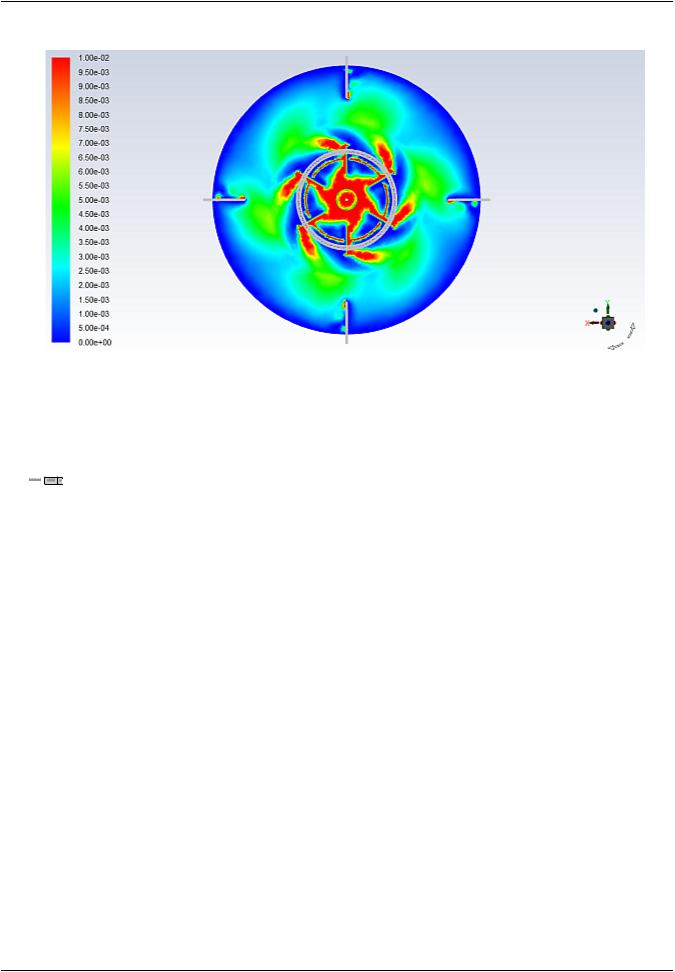
Figure 19.5: Contours of Air Volume Fraction on the z=0.08 plane |
|
Note that the air is collecting on the bottom surface of the Rushton blade turbine disk before its dispersed by the impeller’s blades.
3.Display vectors of velocity magnitude for water on the XZ plane (Figure 19.6: Vectors of Water Velocity Magnitude on the XZ plane (p. 670)).
 Results → Graphics → Vectors → Edit...
a.Select Velocity from the Vectors of drop-down list.
b.Select water from the Phase drop-down list.
Since the Eulerian model solves individual momentum equations for each phase, you can choose the phase for which solution data is plotted.
c.From the Color by drop-down lists, select Velocity... and Velocity Magnitude.
d.Retain the selection of water from the Phase drop-down list.
e.In the Surfaces selection list, deselect all surfaces by clicking  and then select y=0, wall_impeller_1, and wall_impeller_2.
f.Click Display and use the interactive triad to orient the view as shown in Figure 19.6: Vectors of Water Velocity Magnitude on the XZ plane (p. 670).
Release 2019 R1 - © ANSYS,Inc.All rights reserved.- Contains proprietary and confidential information |
|
of ANSYS, Inc. and its subsidiaries and affiliates. |
669 |

vk.com/club152685050Using the Multiphase Models| vk.com/id446425943
Figure 19.6: Vectors of Water Velocity Magnitude on the XZ plane
The vector plot of the water velocity shows that the water moves in a circular motion, creating a closed loop since it cannot escape the reactor.
4.Display vectors of velocity magnitude for air on the XZ plane (Figure 19.7: Vectors of Air Velocity Magnitude on the XZ plane (p. 670)).
a.Under Vectors of, select air from the Phase drop-down list.
b.Under Color by, select air from the Phase drop-down list.
c.In the Surfaces selection list, make sure that y=0, wall_impeller_1, and wall_impeller_2 are selected.
d.Click Display.
Figure 19.7: Vectors of Air Velocity Magnitude on the XZ plane
|
Release 2019 R1 - © ANSYS,Inc.All rights reserved.- Contains proprietary and confidential information |
670 |
of ANSYS, Inc. and its subsidiaries and affiliates. |