vk.com/club152685050 | vk.com/id446425943

Setup and Solution

a.Enter 0.7369 atm for Gauge Pressure.

b.Retain Intensity and Viscosity Ratio from the Specification Method drop-down list in the Turbulence group box.

c.Enter 1.5% for Backflow Turbulent Intensity.

d.Retain the setting of 10 for Backflow Turbulent Viscosity Ratio.

If substantial backflow occurs at the outlet, you may need to adjust the backflow values to levels close to the actual exit conditions.

e.Click OK to close the Pressure Outlet dialog box.

6.4.8. Solution: Steady Flow

In this step, you will generate a steady-state flow solution that will be used as an initial condition for the time-dependent solution.

1. Define the solution parameters.

Release 2019 R1 - © ANSYS,Inc.All rights reserved.- Contains proprietary and confidential information
of ANSYS, Inc. and its subsidiaries and affiliates.	209

vk.com/club152685050Modeling Transient Compressible| vk.com/id446425943Flow

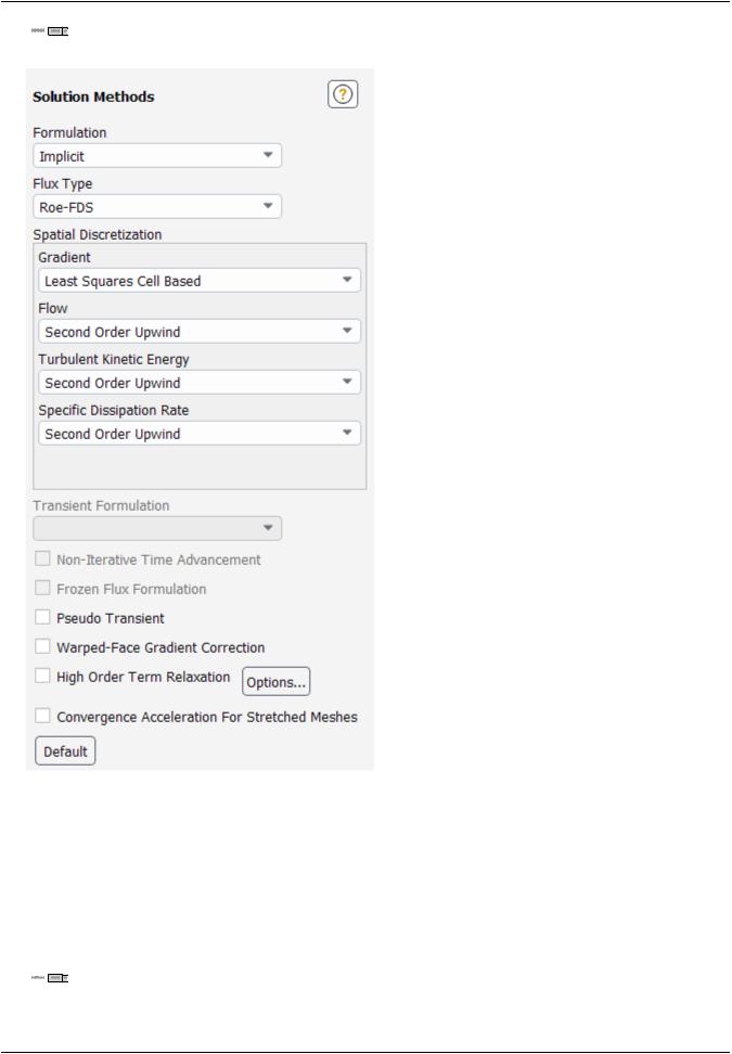
Solution → Solution → Methods...

a.Retain the default selection of Least Squares Cell Based from the Gradient drop-down list in the

Spatial Discretization group box.

b.Select Second Order Upwind from the Turbulent Kinetic Energy and Specific Dissipation Rate dropdown lists.

Second-order discretization provides optimum accuracy.

2.Modify the Courant Number.

Solution → Controls → Controls...

	Release 2019 R1 - © ANSYS,Inc.All rights reserved.- Contains proprietary and confidential information
210	of ANSYS, Inc. and its subsidiaries and affiliates.

vk.com/club152685050 | vk.com/id446425943

Setup and Solution

a. Enter 50 for the Courant Number.

Note

The default Courant number for the density-based implicit formulation is 5. For relatively simple problems, setting the Courant number to 10, 20, 100, or even higher value may be suitable and produce fast and stable convergence. However, if you encounter convergence difficulties at the startup of the simulation of a properly set up problem, then you should consider setting the Courant number to its default value of 5. As the solution progresses, you can start to gradually increase the Courant number until the final convergence is reached.

b.Retain the default values for the Under-Relaxation Factors.

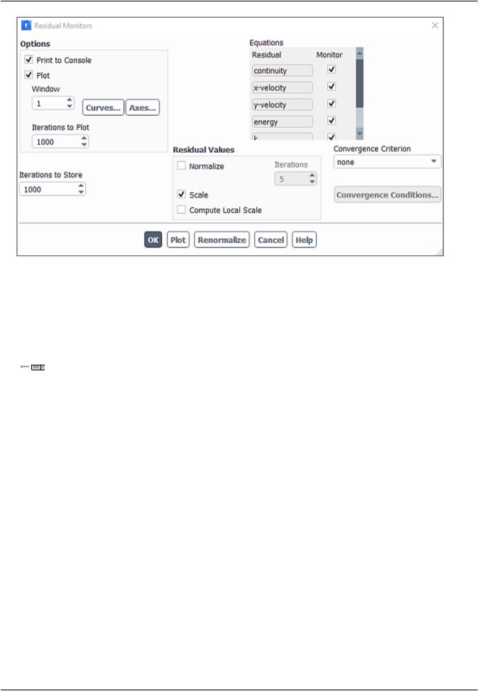
3.Enable the plotting of residuals.

Solution → Reports → Residuals...

Release 2019 R1 - © ANSYS,Inc.All rights reserved.- Contains proprietary and confidential information
of ANSYS, Inc. and its subsidiaries and affiliates.	211

vk.com/club152685050Modeling Transient Compressible| vk.com/id446425943Flow

a.Ensure that Plot is enabled in the Options group box.

b.Select none from the Convergence Criterion drop-down list.

c.Click OK to close the Residual Monitors dialog box.

4.Create the surface report definition for mass flow rate at the flow exit.

Solution → Reports → Definitions → New → Surface Report → Mass Flow Rate...

	Release 2019 R1 - © ANSYS,Inc.All rights reserved.- Contains proprietary and confidential information
212	of ANSYS, Inc. and its subsidiaries and affiliates.

vk.com/club152685050 | vk.com/id446425943

Setup and Solution

a.Enter mass_flowrate_out for Name.

b.Select outlet in the Surfaces selection list.

c.In the Create group box, enable Report File, Report Plot and Print to Console.

Note

When Report File is enabled in the Surface Report Definition dialog box, the mass flow rate history will be written to a file. If you do not enable this option, the history information will be lost when you exit ANSYS Fluent.

d. Click OK to close the Surface Report Definition dialog box.

Release 2019 R1 - © ANSYS,Inc.All rights reserved.- Contains proprietary and confidential information
of ANSYS, Inc. and its subsidiaries and affiliates.	213

vk.com/club152685050Modeling Transient Compressible| vk.com/id446425943Flow

mass_flowrate_out-rplot and mass_flowrate_out-rfile are automatically generated by Fluent and appear in the tree (under Solution/Monitors/Report Plots and Solution/Monitors/Report Files, respectively).

e. Modify the output file name.

Solution → Monitors → Report Files → mass_flowrate_out-rfile Edit...

i.Enter noz_ss.out for Output File Base Name.

ii.Click OK to close the Edit Report File dialog box.

5.Save the case file (noz_ss.cas.gz).

File → Write → Case...

6.Initialize the solution.

Solution → Initialization

	Release 2019 R1 - © ANSYS,Inc.All rights reserved.- Contains proprietary and confidential information
214	of ANSYS, Inc. and its subsidiaries and affiliates.

vk.com/club152685050 | vk.com/id446425943

Setup and Solution

a.Keep the Method at the default of Hybrid.

b.Click Initialize.

7.Set up gradient adaption for dynamic mesh refinement.

You will enable dynamic adaption so that the solver periodically refines the mesh in the vicinity of the shocks as the iterations progress. The shocks are identified by their large pressure gradients.

Domain → Adapt → Refine / Coarsen...

a.Select New and Field Variable... from the Cell Registers drop-down list. Setup the refinement cell regsiter.

Release 2019 R1 - © ANSYS,Inc.All rights reserved.- Contains proprietary and confidential information
of ANSYS, Inc. and its subsidiaries and affiliates.	215

vk.com/club152685050Modeling Transient Compressible| vk.com/id446425943Flow

i.Select Cells More Than from the Type drop-down list.

ii.Select Gradient from the Deriviative Option drop-down list.

iii.Select Scale by Global Average from the Scaling Option drop-down list.

iv.Select Pressure... and Static Pressure from the Curvature of drop down list.

v.Click Compute.

ANSYS Fluent will update the Min and Max values to show the minimum and maximum pressure gradient.

vi.Enter a value of 0.7 for the Cells having value more than field.

vii.Enter scaled_gradient_refn for the Name of this Field Variable Register.

viii.Click Save.

ix.Click Close to close the Field Variable Register dialog box.

Setup the coarsening cell regsiter.

i.Select Cells Less Than from the Type drop-down list.

ii.Select Gradient from the Deriviative Option drop-down list.

iii.Select Scale by Global Average from the Scaling Option drop down list.

iv.Select Pressure... and Static Pressure from the Curvature of drop-down list.

v.Click Compute.

ANSYS Fluent will update the Min and Max values to show the minimum and maximum pressure gradient.

vi.Enter a value of 0.3 for the Cells having value less than field.

vii.Enter scaled_gradient_crsn for the Name of this Field Variable Register.

	Release 2019 R1 - © ANSYS,Inc.All rights reserved.- Contains proprietary and confidential information
216	of ANSYS, Inc. and its subsidiaries and affiliates.

vk.com/club152685050 | vk.com/id446425943

Setup and Solution

viii.Click Save.

ix.Click Close to close the Field Variable Register dialog box.

The mesh adaption criterion can either be the gradient or the curvature (second gradient). Because strong shocks occur inside the nozzle, the gradient is used as the adaption criterion.

b. In the Adaption Controls dialog box select the refinement and coaresning criterion.

i.Select scaled_gradient_refn from the Refinement Criterion drop-down list.

ii.Select scaled_gradient_crsn from the Coarsening Criterion drop-down list.

iii.Enable Dynamic Adaption.

iv.Enter 100 for Frequency (iteration) of mesh adaption.

v.Click OK to close the Adaption Controls dialog box.

8.Start the calculation by requesting 500 iterations.

Solution → Run Calculation → Advanced...

Release 2019 R1 - © ANSYS,Inc.All rights reserved.- Contains proprietary and confidential information
of ANSYS, Inc. and its subsidiaries and affiliates.	217

vk.com/club152685050Modeling Transient Compressible| vk.com/id446425943Flow

a.Enter 500 for Number of Iterations.

b.Click Calculate to start the steady flow simulation.

Figure 6.3: Mass Flow Rate History

	Release 2019 R1 - © ANSYS,Inc.All rights reserved.- Contains proprietary and confidential information
218	of ANSYS, Inc. and its subsidiaries and affiliates.

vk.com/club152685050 | vk.com/id446425943

Setup and Solution

9.Save the case and data files (noz_ss.cas.gz and noz_ss.dat.gz).

File → Write → Case & Data...

Note

When you write the case and data files at the same time, it does not matter whether you specify the file name with a .cas or .dat extension, as both will be saved.

10.Click OK in the Question dialog box to overwrite the existing file.

11.Review a mesh that resulted from the dynamic adaption performed during the computation.

Results → Graphics → Mesh Edit...

a.Ensure that only the Edges option is enabled in the Options group box.

b.Select Feature from the Edge Type list.

c.Ensure that all of the items are selected from the Surfaces selection list.

d.Click Display and close the Mesh Display dialog box.

The mesh after adaption is displayed in the graphics window (Figure 6.4: 2D Nozzle Mesh after Adaption (p. 220))

Release 2019 R1 - © ANSYS,Inc.All rights reserved.- Contains proprietary and confidential information
of ANSYS, Inc. and its subsidiaries and affiliates.	219

vk.com/club152685050Modeling Transient Compressible| vk.com/id446425943Flow

Figure 6.4: 2D Nozzle Mesh after Adaption

e.Zoom in using the middle mouse button to view aspects of your mesh.

Notice that the cells in the regions of high pressure gradients have been refined.

12.Display the steady flow contours of static pressure (Figure 6.5: Contours of Static Pressure (Steady Flow) (p. 221)).

Results → Graphics → Contours → Edit...

	Release 2019 R1 - © ANSYS,Inc.All rights reserved.- Contains proprietary and confidential information
220	of ANSYS, Inc. and its subsidiaries and affiliates.

vk.com/club152685050 | vk.com/id446425943

Setup and Solution

a.Enable Filled in the Options group box.

b.Click Display and close the Contours dialog box.

Figure 6.5: Contours of Static Pressure (Steady Flow)

Release 2019 R1 - © ANSYS,Inc.All rights reserved.- Contains proprietary and confidential information
of ANSYS, Inc. and its subsidiaries and affiliates.	221

vk.com/club152685050Modeling Transient Compressible| vk.com/id446425943Flow

The steady flow prediction in Figure 6.5: Contours of Static Pressure (Steady Flow) (p. 221) shows the expected pressure distribution, with low pressure near the nozzle throat.

13.Display the steady-flow velocity vectors (Figure 6.6: Velocity Vectors Showing Recirculation (Steady Flow) (p. 223)).

Results → Graphics → Vectors → Edit...

a.Enter 2 under Scale.

b.Click Display and close the Vectors dialog box.

The steady flow prediction shows the expected form, with a peak velocity of approximately 300 m/s through the nozzle.

You can zoom in on the wall in the expansion region of the nozzle to view the recirculation of the flow as shown in Figure 6.6: Velocity Vectors Showing Recirculation (Steady Flow) (p. 223) .

	Release 2019 R1 - © ANSYS,Inc.All rights reserved.- Contains proprietary and confidential information
222	of ANSYS, Inc. and its subsidiaries and affiliates.

vk.com/club152685050 | vk.com/id446425943

Setup and Solution

Figure 6.6: Velocity Vectors Showing Recirculation (Steady Flow)

14. Check the mass flux balance.

Important

Although the mass flow rate history indicates that the solution is converged, you should also check the mass flux throughout the domain to ensure that mass is being conserved.

Results → Reports → Fluxes...

a.Retain the default selection of Mass Flow Rate.

b.Select inlet and outlet in the Boundaries selection list.

Release 2019 R1 - © ANSYS,Inc.All rights reserved.- Contains proprietary and confidential information
of ANSYS, Inc. and its subsidiaries and affiliates.	223