vk.com/club152685050 | vk.com/id446425943

Setup and Solution

Setup → Boundary Conditions → wall-6 Edit...

Note

A Stationary Wall condition implies that the wall is stationary with respect to the adjacent cell zone. Hence, in the case of a rotating reference frame a Stationary Wall is actually rotating with respect to the absolute reference frame. To specify a non-rotating wall in this case you would select Moving Wall (that is, moving with respect to the rotating reference frame). Then you would specify an absolute rotational speed of 0 in the Motion group box.

a. Click OK to close the Wall dialog box.

9.4.8. Solution Using the Standard k- ε Model

1.Set the solution parameters.

Solution → Solution → Methods...

Release 2019 R1 - © ANSYS,Inc.All rights reserved.- Contains proprietary and confidential information
of ANSYS, Inc. and its subsidiaries and affiliates.	329

vk.com/club152685050Using a Single Rotating Reference| vk.com/id446425943Frame

a.Select PRESTO! from the Pressure drop-down list in the Spatial Discretization group box.

The PRESTO! scheme is well suited for steep pressure gradients involved in rotating flows. It provides improved pressure interpolation in situations where large body forces or strong pressure variations are present as in swirling flows.

b.Select Second Order Upwind from the Turbulent Kinetic Energy and Turbulent Dissipation Rate drop-down lists.

Use the scroll bar to access the discretization schemes that are not initially visible in the task page.

2.Set the solution controls.

Solution → Controls → Controls...

	Release 2019 R1 - © ANSYS,Inc.All rights reserved.- Contains proprietary and confidential information
330	of ANSYS, Inc. and its subsidiaries and affiliates.

vk.com/club152685050 | vk.com/id446425943

Setup and Solution

a. Retain the default values in the Pseudo Transient Explicit Relaxation Factors group box.

Note

For this problem, the default explicit relaxation factors are satisfactory. However, if

the solution diverges or the residuals display large oscillations, you may need to reduce the relaxation factors from their default values.

For tips on how to adjust the explicit relaxation parameters for different situations, see the Fluent User's Guide.

3.Enable the plotting of residuals during the calculation.

Solution → Reports → Residuals...

Release 2019 R1 - © ANSYS,Inc.All rights reserved.- Contains proprietary and confidential information
of ANSYS, Inc. and its subsidiaries and affiliates.	331

vk.com/club152685050Using a Single Rotating Reference| vk.com/id446425943Frame

a.Ensure that Plot is enabled in the Options group box.

b.Click OK to close the Residual Monitors dialog box.

Note

For this calculation, the convergence tolerance on the continuity equation is kept at 0.001. Depending on the behavior of the solution, you can reduce this value if necessary.

4.Enable the plotting of mass flow rate at the flow exit.

Solution → Reports → Definitions → New → Surface Report → Mass Flow Rate

	Release 2019 R1 - © ANSYS,Inc.All rights reserved.- Contains proprietary and confidential information
332	of ANSYS, Inc. and its subsidiaries and affiliates.

vk.com/club152685050 | vk.com/id446425943

Setup and Solution

a.Enter surf-mon-1 for the Name of the surface report definition.

b.In the Create group box, enable Report File, Report Plot and Print to Console for surf-mon-1.

Note

When the Report File option is selected in the Surface Report Definition dialog box, the mass flow rate history will be written to a file. If you do not enable the Report File option, the history information will be lost when you exit ANSYS Fluent.

c.Select pressure-outlet-3 from the Surfaces selection list.

d.Click OK to save the surface report definition settings and close the Surface Report Definition dialog box.

5.Initialize the solution.

Release 2019 R1 - © ANSYS,Inc.All rights reserved.- Contains proprietary and confidential information
of ANSYS, Inc. and its subsidiaries and affiliates.	333

vk.com/club152685050Using a Single Rotating Reference| vk.com/id446425943Frame

Solution → Initialization

a.Retain the default selection of the Hybrid initialization method.

b.Click Initialize.

Note

For flows in complex topologies, hybrid initialization will provide better initial velocity and pressure fields than standard initialization. This in general will help in improving the convergence behavior of the solver.

6.Save the case file (disk-ke.cas.gz).

File → Write → Case...

7.Start the calculation by requesting 600 iterations.

Run Calculation

a.Enter 600 for the Number of Iterations.

b.Click Calculate.

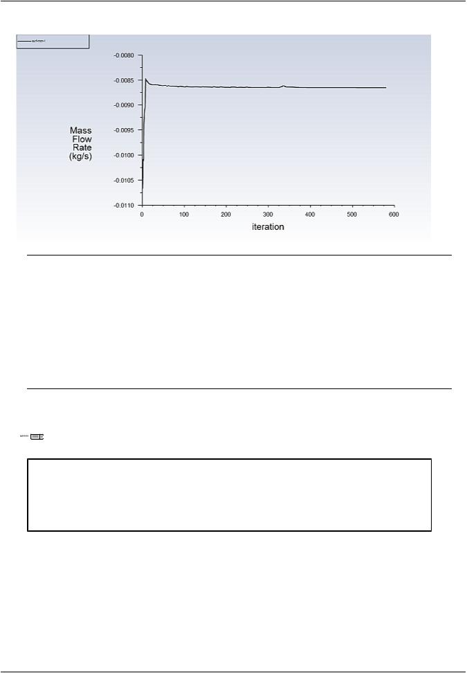
Throughout the calculation, ANSYS Fluent will report reversed flow at the exit. This is reasonable for the current case. The mass flow rate history is shown in Figure 9.3: Mass Flow Rate History (k- ε Tur- bulence Model) (p. 335).

	Release 2019 R1 - © ANSYS,Inc.All rights reserved.- Contains proprietary and confidential information
334	of ANSYS, Inc. and its subsidiaries and affiliates.

vk.com/club152685050 | vk.com/id446425943

Setup and Solution

Figure 9.3: Mass Flow Rate History (k- ε Turbulence Model)

Extra

Here we have retained the default Timescale Factor of 1 in the Run Calculation panel. When performing a Pseudo Transient calculation, larger values of Timescale Factor may speed up convergence of the solution. However, setting Timescale Factor too large may cause the solution to diverge and fail to complete. As an optional activity, you can reinitialize the solution and try running the calculation with Timescale Factor set to 2. Observe the convergence behavior and the number of iterations before convergence. Then try the same again with Timescale Factor set to 4. For more information on setting Timescale Factor and the Pseudo Transient solver settings, refer to the Fluent User's Guide.

8.Check the mass flux balance.

Results → Reports → Fluxes...

Warning

Although the mass flow rate history indicates that the solution is converged, you should also check the net mass fluxes through the domain to ensure that mass is being conserved.

Release 2019 R1 - © ANSYS,Inc.All rights reserved.- Contains proprietary and confidential information
of ANSYS, Inc. and its subsidiaries and affiliates.	335