vk.com/club152685050Modeling Species Transport| vkand.com/id446425943Gaseous Combustion

excess air). The high-speed methane jet initially expands with little interference from the outer wall, and entrains and mixes with the low-speed air. The Reynolds number based on the methane jet diameter is approximately .

Figure 13.1: Combustion of Methane Gas in a Turbulent Diffusion Flame Furnace

13.4. Background

In this tutorial, you will use the generalized eddy-dissipation model to analyze the methane-air combustion system. The combustion will be modeled using a global one-step reaction mechanism, assuming complete conversion of the fuel to and . The reaction equation is

(13.1)

This reaction will be defined in terms of stoichiometric coefficients, formation enthalpies, and parameters that control the reaction rate. The reaction rate will be determined assuming that turbulent mixing is the rate-limiting process, with the turbulence-chemistry interaction modeled using the eddy-dissipation model.

13.5. Setup and Solution

The following sections describe the setup and solution steps for this tutorial:

13.5.1.Preparation

13.5.2.Mesh

13.5.3.General Settings

13.5.4.Models

13.5.5.Materials

13.5.6.Boundary Conditions

13.5.7.Initial Reaction Solution

13.5.8.Postprocessing

13.5.9.NOx Prediction

13.5.1. Preparation

To prepare for running this tutorial:

1.Download the species_transport.zip file here.

2.Unzip species_transport.zip to your working directory.

3.The file gascomb.msh can be found in the folder.

4.Use Fluent Launcher to start the 2D version of ANSYS Fluent.

	Release 2019 R1 - © ANSYS,Inc.All rights reserved.- Contains proprietary and confidential information
444	of ANSYS, Inc. and its subsidiaries and affiliates.

vk.com/club152685050 | vk.com/id446425943

Setup and Solution

Fluent Launcher displays your Display Options preferences from the previous session.

For more information about Fluent Launcher, see starting ANSYS Fluent using the Fluent Launcher in the Fluent Getting Started Guide.

5.Ensure that the Display Mesh After Reading option is enabled.

6.Enable Double-Precision.

7.Ensure Serial is selected under Processing Options.

13.5.2. Mesh

1. Read the mesh file gascomb.msh.

File → Read → Mesh...

13.5.3. General Settings

1.Check the mesh.

Domain → Mesh → Check → Perform Mesh Check

ANSYS Fluent will perform various checks on the mesh and will report the progress in the console. Ensure that the reported minimum volume reported is a positive number.

2.Scale the mesh.

Domain → Mesh → Scale...

Since this mesh was created in units of millimeters, you will need to scale the mesh into meters.

a. Select mm from the Mesh Was Created In drop-down list in the Scaling group box.

Release 2019 R1 - © ANSYS,Inc.All rights reserved.- Contains proprietary and confidential information
of ANSYS, Inc. and its subsidiaries and affiliates.	445

vk.com/club152685050Modeling Species Transport| vkand.com/id446425943Gaseous Combustion

b.Click Scale.

c.Ensure that m is selected from the View Length Unit In drop-down list.

d.Ensure that Xmax and Ymax are reset to 1.8 m and 0.225 m respectively.

The default SI units will be used in this tutorial, hence there is no need to change any units in this problem.

e.Close the Scale Mesh dialog box.

f.Right click in the graphics window and select Refresh Display

g.Clicking the Fit to Window icon, , will cause the object to fit exactly and be centered in the window.

3.Check the mesh.

Domain → Mesh → Check → Perform Mesh Check

Note

You should check the mesh after you manipulate it (scale, convert to polyhedra, merge, separate, fuse, add zones, or smooth and swap). This will ensure that the quality of the mesh has not been compromised.

4.Examine the mesh with the default settings.

Figure 13.2: The Quadrilateral Mesh for the Combustor Model

Extra

You can use the right mouse button to probe for mesh information in the graphics window. If you click the right mouse button on any node in the mesh, information will be displayed in the ANSYS Fluent console about the associated zone, including the name of

	Release 2019 R1 - © ANSYS,Inc.All rights reserved.- Contains proprietary and confidential information
446	of ANSYS, Inc. and its subsidiaries and affiliates.

vk.com/club152685050 | vk.com/id446425943

Setup and Solution

the zone. This feature is especially useful when you have several zones of the same type and you want to distinguish between them quickly.

5.Select Axisymmetric in the 2D Space list.

Setup → General

13.5.4. Models

1.Enable heat transfer by enabling the energy equation.

Physics → Models → Energy

2. Select the standard - turbulence model.

Release 2019 R1 - © ANSYS,Inc.All rights reserved.- Contains proprietary and confidential information
of ANSYS, Inc. and its subsidiaries and affiliates.	447

vk.com/club152685050Modeling Species Transport| vkand.com/id446425943Gaseous Combustion

Physics → Models → Viscous...

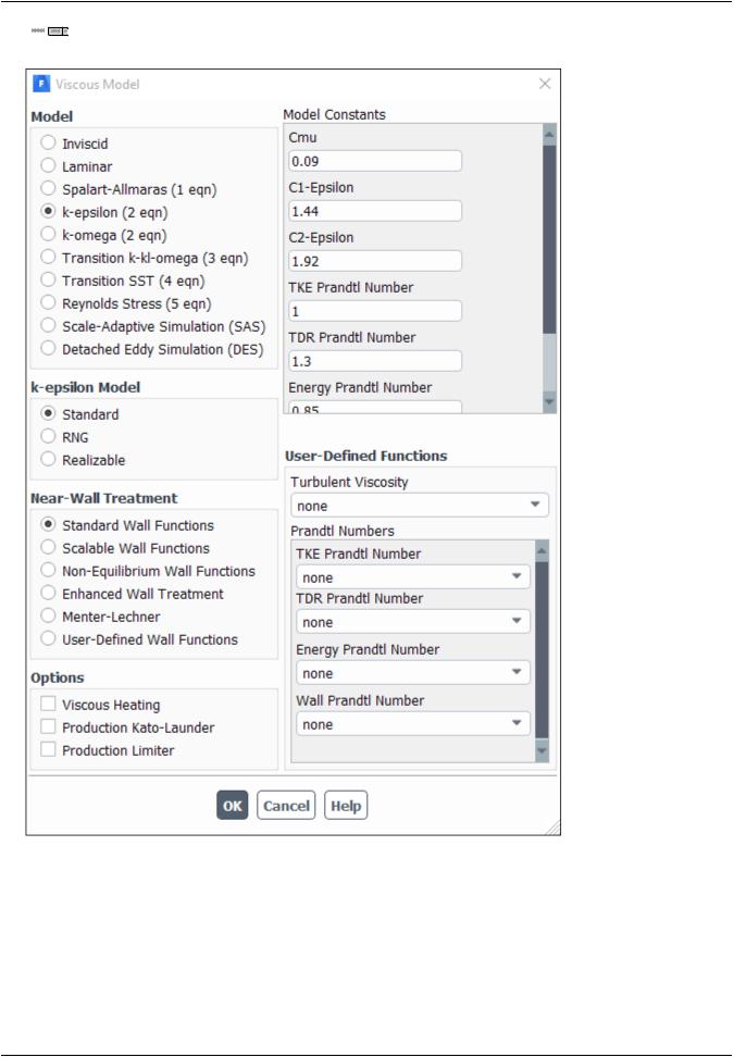
a.Select k-epsilon (2 eqn) in the Model list.

The Viscous Model dialog box will expand to provide further options for the k-epsilon model.

b.Retain the default settings for the k-epsilon model.

c.Click OK to close the Viscous Model dialog box.

3.Enable chemical species transport and reaction.

	Release 2019 R1 - © ANSYS,Inc.All rights reserved.- Contains proprietary and confidential information
448	of ANSYS, Inc. and its subsidiaries and affiliates.

vk.com/club152685050 | vk.com/id446425943

Setup and Solution

Physics → Models → Species...

a.Select Species Transport in the Model list.

The Species Model dialog box will expand to provide further options for the Species Transport model.

b.Enable Volumetric in the Reactions group box.

c.Select methane-air from the Mixture Material drop-down list.

Scroll down the list to find methane-air.

Note

The Mixture Material list contains the set of chemical mixtures that exist in the ANSYS Fluent database. You can select one of the predefined mixtures to access a complete description of the reacting system. The chemical species in the system and their

Release 2019 R1 - © ANSYS,Inc.All rights reserved.- Contains proprietary and confidential information
of ANSYS, Inc. and its subsidiaries and affiliates.	449