vk.com/club152685050Modeling Transient Compressible| vk.com/id446425943Flow

c. Click Compute and examine the values displayed in the dialog box.

Important

The net mass imbalance should be a small fraction (for example, 0.1%) of the total flux through the system. The imbalance is displayed in the lower right field under Net Results. If a significant imbalance occurs, you should decrease your residual tolerances by at least an order of magnitude and continue iterating.

d. Close the Flux Reports dialog box.

6.4.9. Enabling Time Dependence and Setting Transient Conditions

In this step you will define a transient flow by specifying a transient pressure condition for the nozzle.

1.Enable a time-dependent flow calculation.

Physics → Solver → Transient

2.Read the user-defined function (pexit.c), in preparation for defining the transient condition for the nozzle exit.

The pressure at the outlet is defined as a wave-shaped profile, and is described by the following equation:

(6.1)

where

= circular frequency of transient pressure (rad/s)

	= mean exit pressure (atm)
In this case,	rad/s, and	atm.

A user-defined function ( pexit.c ) has been written to define the equation (Equation 6.1 (p. 224)) required for the pressure profile.

Note

To input the value of Equation 6.1 (p. 224) in the correct units, the function pexit.c has to be written in SI units.

More details about user-defined functions can be found in the Fluent Customization Manual.

User-Defined → User Defined → Functions → Interpreted...

	Release 2019 R1 - © ANSYS,Inc.All rights reserved.- Contains proprietary and confidential information
224	of ANSYS, Inc. and its subsidiaries and affiliates.

vk.com/club152685050 | vk.com/id446425943

Setup and Solution

a.Enter pexit.c for Source File Name.

If the UDF source file is not in your working directory, then you must enter the entire directory path for Source File Name instead of just entering the file name.

b.Click Interpret.

The user-defined function has already been defined, but it must be compiled within ANSYS Fluent before it can be used in the solver.

c.Close the Interpreted UDFs dialog box.

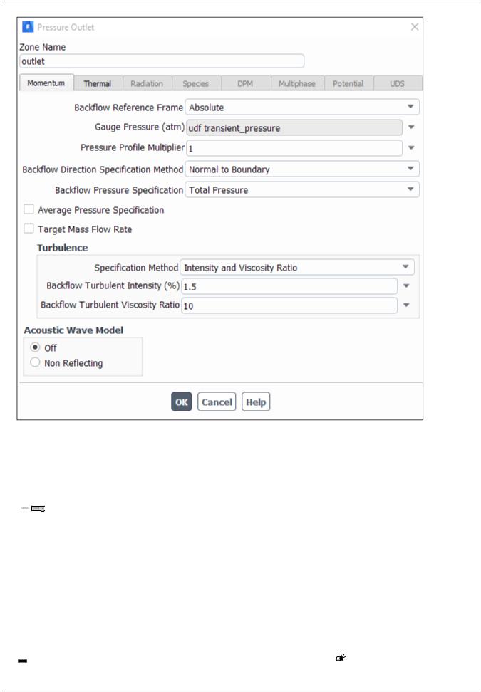
3.Define the transient boundary conditions at the nozzle exit (outlet).

Setup → Boundary Conditions → outlet Edit...

Release 2019 R1 - © ANSYS,Inc.All rights reserved.- Contains proprietary and confidential information
of ANSYS, Inc. and its subsidiaries and affiliates.	225

vk.com/club152685050Modeling Transient Compressible| vk.com/id446425943Flow

a.Select udf transient_pressure (the user-defined function) from the Gauge Pressure drop-down list.

b.Click OK to close the Pressure Outlet dialog box.

4.Update the gradient adaption parameters for the transient case.

Domain → Adapt → Refine / Coarsen...

a.Enter 10 for Interval in the Dynamic group box.

For the transient case, the mesh adaption will be done every 10 time steps.

b.Click Ok to close the Adaption Controls dialog box.

6.4.10. Specifying Solution Parameters for Transient Flow and Solving

1. Modify the mass_flowrate_out-rfile report file definition.

Solution → Monitors → Report Files → mass_flowrate_out-rfile Edit...

	Release 2019 R1 - © ANSYS,Inc.All rights reserved.- Contains proprietary and confidential information
226	of ANSYS, Inc. and its subsidiaries and affiliates.

vk.com/club152685050 | vk.com/id446425943

Setup and Solution

a.Enter noz_uns.out for Output File Base Name.

b.Select time-step from the Get Data Every drop-down list.

c.Click OK to close the Edit Report File dialog box.

2.Modify the mass_flowrate_out-rplot report plot definition.

Solution → Monitors → Report Plots → mass_flowrate_out-rplot Edit...

Release 2019 R1 - © ANSYS,Inc.All rights reserved.- Contains proprietary and confidential information
of ANSYS, Inc. and its subsidiaries and affiliates.	227

vk.com/club152685050Modeling Transient Compressible| vk.com/id446425943Flow

a.For Get Data Every, retain the value of 1 and select time-step from the drop-down list.

Because each time step requires 10 iterations, a smoother plot will be generated by plotting at every time step.

b.Select time-step from the X-Axis Label drop-down list.

c.Click OK to close the Edit Report File dialog box.

3.Save the transient solution case file (noz_uns.cas.gz).

File → Write → Case...

4.Modify the plotting of residuals.

Solution → Reports → Residuals...

a.Ensure that Plot is enabled in the Options group box.

b.Ensure none is selected from the Convergence Criterion drop-down list.

c.Set the Iterations to Plot to 100.

d.Click OK to close the Residual Monitors dialog box.

	Release 2019 R1 - © ANSYS,Inc.All rights reserved.- Contains proprietary and confidential information
228	of ANSYS, Inc. and its subsidiaries and affiliates.

vk.com/club152685050 | vk.com/id446425943

Setup and Solution

5.Define the time step parameters.

The selection of the time step is critical for accurate time-dependent flow predictions. Using a time step of 2.85596 x 10-5 seconds, 100 time steps are required for one pressure cycle. The pressure cycle begins and ends with the initial pressure at the nozzle exit.

Solution → Run Calculation → Advanced

a.Enter 2.85596e-5 s for Time Step Size.

b.Enter 600 for Number of Time Steps.

c.Enter 10 for Max Iterations/Time Step.

d.Click Calculate to start the transient simulation.

Release 2019 R1 - © ANSYS,Inc.All rights reserved.- Contains proprietary and confidential information
of ANSYS, Inc. and its subsidiaries and affiliates.	229