

- •ANSYS Fluent Tutorial Guide
- •Table of Contents
- •Using This Manual
- •1. What’s In This Manual
- •2. How To Use This Manual
- •2.1. For the Beginner
- •2.2. For the Experienced User
- •3. Typographical Conventions Used In This Manual
- •Chapter 1: Fluid Flow in an Exhaust Manifold
- •1.1. Introduction
- •1.2. Prerequisites
- •1.3. Problem Description
- •1.4. Setup and Solution
- •1.4.1. Preparation
- •1.4.2. Meshing Workflow
- •1.4.3. General Settings
- •1.4.4. Solver Settings
- •1.4.5. Models
- •1.4.6. Materials
- •1.4.7. Cell Zone Conditions
- •1.4.8. Boundary Conditions
- •1.4.9. Solution
- •1.4.10. Postprocessing
- •1.5. Summary
- •Chapter 2: Fluid Flow and Heat Transfer in a Mixing Elbow
- •2.1. Introduction
- •2.2. Prerequisites
- •2.3. Problem Description
- •2.4. Setup and Solution
- •2.4.1. Preparation
- •2.4.2. Launching ANSYS Fluent
- •2.4.3. Reading the Mesh
- •2.4.4. Setting Up Domain
- •2.4.5. Setting Up Physics
- •2.4.6. Solving
- •2.4.7. Displaying the Preliminary Solution
- •2.4.8. Adapting the Mesh
- •2.5. Summary
- •Chapter 3: Postprocessing
- •3.1. Introduction
- •3.2. Prerequisites
- •3.3. Problem Description
- •3.4. Setup and Solution
- •3.4.1. Preparation
- •3.4.2. Reading the Mesh
- •3.4.3. Manipulating the Mesh in the Viewer
- •3.4.4. Adding Lights
- •3.4.5. Creating Isosurfaces
- •3.4.6. Generating Contours
- •3.4.7. Generating Velocity Vectors
- •3.4.8. Creating an Animation
- •3.4.9. Displaying Pathlines
- •3.4.10. Creating a Scene With Vectors and Contours
- •3.4.11. Advanced Overlay of Pathlines on a Scene
- •3.4.12. Creating Exploded Views
- •3.4.13. Animating the Display of Results in Successive Streamwise Planes
- •3.4.14. Generating XY Plots
- •3.4.15. Creating Annotation
- •3.4.16. Saving Picture Files
- •3.4.17. Generating Volume Integral Reports
- •3.5. Summary
- •Chapter 4: Modeling Periodic Flow and Heat Transfer
- •4.1. Introduction
- •4.2. Prerequisites
- •4.3. Problem Description
- •4.4. Setup and Solution
- •4.4.1. Preparation
- •4.4.2. Mesh
- •4.4.3. General Settings
- •4.4.4. Models
- •4.4.5. Materials
- •4.4.6. Cell Zone Conditions
- •4.4.7. Periodic Conditions
- •4.4.8. Boundary Conditions
- •4.4.9. Solution
- •4.4.10. Postprocessing
- •4.5. Summary
- •4.6. Further Improvements
- •Chapter 5: Modeling External Compressible Flow
- •5.1. Introduction
- •5.2. Prerequisites
- •5.3. Problem Description
- •5.4. Setup and Solution
- •5.4.1. Preparation
- •5.4.2. Mesh
- •5.4.3. Solver
- •5.4.4. Models
- •5.4.5. Materials
- •5.4.6. Boundary Conditions
- •5.4.7. Operating Conditions
- •5.4.8. Solution
- •5.4.9. Postprocessing
- •5.5. Summary
- •5.6. Further Improvements
- •Chapter 6: Modeling Transient Compressible Flow
- •6.1. Introduction
- •6.2. Prerequisites
- •6.3. Problem Description
- •6.4. Setup and Solution
- •6.4.1. Preparation
- •6.4.2. Reading and Checking the Mesh
- •6.4.3. Solver and Analysis Type
- •6.4.4. Models
- •6.4.5. Materials
- •6.4.6. Operating Conditions
- •6.4.7. Boundary Conditions
- •6.4.8. Solution: Steady Flow
- •6.4.9. Enabling Time Dependence and Setting Transient Conditions
- •6.4.10. Specifying Solution Parameters for Transient Flow and Solving
- •6.4.11. Saving and Postprocessing Time-Dependent Data Sets
- •6.5. Summary
- •6.6. Further Improvements
- •Chapter 7: Modeling Flow Through Porous Media
- •7.1. Introduction
- •7.2. Prerequisites
- •7.3. Problem Description
- •7.4. Setup and Solution
- •7.4.1. Preparation
- •7.4.2. Mesh
- •7.4.3. General Settings
- •7.4.4. Models
- •7.4.5. Materials
- •7.4.6. Cell Zone Conditions
- •7.4.7. Boundary Conditions
- •7.4.8. Solution
- •7.4.9. Postprocessing
- •7.5. Summary
- •7.6. Further Improvements
- •Chapter 8: Modeling Radiation and Natural Convection
- •8.1. Introduction
- •8.2. Prerequisites
- •8.3. Problem Description
- •8.4. Setup and Solution
- •8.4.1. Preparation
- •8.4.2. Reading and Checking the Mesh
- •8.4.3. Solver and Analysis Type
- •8.4.4. Models
- •8.4.5. Defining the Materials
- •8.4.6. Operating Conditions
- •8.4.7. Boundary Conditions
- •8.4.8. Obtaining the Solution
- •8.4.9. Postprocessing
- •8.4.10. Comparing the Contour Plots after Varying Radiating Surfaces
- •8.4.11. S2S Definition, Solution, and Postprocessing with Partial Enclosure
- •8.5. Summary
- •8.6. Further Improvements
- •Chapter 9: Using a Single Rotating Reference Frame
- •9.1. Introduction
- •9.2. Prerequisites
- •9.3. Problem Description
- •9.4. Setup and Solution
- •9.4.1. Preparation
- •9.4.2. Mesh
- •9.4.3. General Settings
- •9.4.4. Models
- •9.4.5. Materials
- •9.4.6. Cell Zone Conditions
- •9.4.7. Boundary Conditions
- •9.4.8. Solution Using the Standard k- ε Model
- •9.4.9. Postprocessing for the Standard k- ε Solution
- •9.4.10. Solution Using the RNG k- ε Model
- •9.4.11. Postprocessing for the RNG k- ε Solution
- •9.5. Summary
- •9.6. Further Improvements
- •9.7. References
- •Chapter 10: Using Multiple Reference Frames
- •10.1. Introduction
- •10.2. Prerequisites
- •10.3. Problem Description
- •10.4. Setup and Solution
- •10.4.1. Preparation
- •10.4.2. Mesh
- •10.4.3. Models
- •10.4.4. Materials
- •10.4.5. Cell Zone Conditions
- •10.4.6. Boundary Conditions
- •10.4.7. Solution
- •10.4.8. Postprocessing
- •10.5. Summary
- •10.6. Further Improvements
- •Chapter 11: Using Sliding Meshes
- •11.1. Introduction
- •11.2. Prerequisites
- •11.3. Problem Description
- •11.4. Setup and Solution
- •11.4.1. Preparation
- •11.4.2. Mesh
- •11.4.3. General Settings
- •11.4.4. Models
- •11.4.5. Materials
- •11.4.6. Cell Zone Conditions
- •11.4.7. Boundary Conditions
- •11.4.8. Operating Conditions
- •11.4.9. Mesh Interfaces
- •11.4.10. Solution
- •11.4.11. Postprocessing
- •11.5. Summary
- •11.6. Further Improvements
- •Chapter 12: Using Overset and Dynamic Meshes
- •12.1. Prerequisites
- •12.2. Problem Description
- •12.3. Preparation
- •12.4. Mesh
- •12.5. Overset Interface Creation
- •12.6. Steady-State Case Setup
- •12.6.1. General Settings
- •12.6.2. Models
- •12.6.3. Materials
- •12.6.4. Operating Conditions
- •12.6.5. Boundary Conditions
- •12.6.6. Reference Values
- •12.6.7. Solution
- •12.7. Unsteady Setup
- •12.7.1. General Settings
- •12.7.2. Compile the UDF
- •12.7.3. Dynamic Mesh Settings
- •12.7.4. Report Generation for Unsteady Case
- •12.7.5. Run Calculations for Unsteady Case
- •12.7.6. Overset Solution Checking
- •12.7.7. Postprocessing
- •12.7.8. Diagnosing an Overset Case
- •12.8. Summary
- •Chapter 13: Modeling Species Transport and Gaseous Combustion
- •13.1. Introduction
- •13.2. Prerequisites
- •13.3. Problem Description
- •13.4. Background
- •13.5. Setup and Solution
- •13.5.1. Preparation
- •13.5.2. Mesh
- •13.5.3. General Settings
- •13.5.4. Models
- •13.5.5. Materials
- •13.5.6. Boundary Conditions
- •13.5.7. Initial Reaction Solution
- •13.5.8. Postprocessing
- •13.5.9. NOx Prediction
- •13.6. Summary
- •13.7. Further Improvements
- •Chapter 14: Using the Eddy Dissipation and Steady Diffusion Flamelet Combustion Models
- •14.1. Introduction
- •14.2. Prerequisites
- •14.3. Problem Description
- •14.4. Setup and Solution
- •14.4.1. Preparation
- •14.4.2. Mesh
- •14.4.3. Solver Settings
- •14.4.4. Models
- •14.4.5. Boundary Conditions
- •14.4.6. Solution
- •14.4.7. Postprocessing for the Eddy-Dissipation Solution
- •14.5. Steady Diffusion Flamelet Model Setup and Solution
- •14.5.1. Models
- •14.5.2. Boundary Conditions
- •14.5.3. Solution
- •14.5.4. Postprocessing for the Steady Diffusion Flamelet Solution
- •14.6. Summary
- •Chapter 15: Modeling Surface Chemistry
- •15.1. Introduction
- •15.2. Prerequisites
- •15.3. Problem Description
- •15.4. Setup and Solution
- •15.4.1. Preparation
- •15.4.2. Reading and Checking the Mesh
- •15.4.3. Solver and Analysis Type
- •15.4.4. Specifying the Models
- •15.4.5. Defining Materials and Properties
- •15.4.6. Specifying Boundary Conditions
- •15.4.7. Setting the Operating Conditions
- •15.4.8. Simulating Non-Reacting Flow
- •15.4.9. Simulating Reacting Flow
- •15.4.10. Postprocessing the Solution Results
- •15.5. Summary
- •15.6. Further Improvements
- •Chapter 16: Modeling Evaporating Liquid Spray
- •16.1. Introduction
- •16.2. Prerequisites
- •16.3. Problem Description
- •16.4. Setup and Solution
- •16.4.1. Preparation
- •16.4.2. Mesh
- •16.4.3. Solver
- •16.4.4. Models
- •16.4.5. Materials
- •16.4.6. Boundary Conditions
- •16.4.7. Initial Solution Without Droplets
- •16.4.8. Creating a Spray Injection
- •16.4.9. Solution
- •16.4.10. Postprocessing
- •16.5. Summary
- •16.6. Further Improvements
- •Chapter 17: Using the VOF Model
- •17.1. Introduction
- •17.2. Prerequisites
- •17.3. Problem Description
- •17.4. Setup and Solution
- •17.4.1. Preparation
- •17.4.2. Reading and Manipulating the Mesh
- •17.4.3. General Settings
- •17.4.4. Models
- •17.4.5. Materials
- •17.4.6. Phases
- •17.4.7. Operating Conditions
- •17.4.8. User-Defined Function (UDF)
- •17.4.9. Boundary Conditions
- •17.4.10. Solution
- •17.4.11. Postprocessing
- •17.5. Summary
- •17.6. Further Improvements
- •Chapter 18: Modeling Cavitation
- •18.1. Introduction
- •18.2. Prerequisites
- •18.3. Problem Description
- •18.4. Setup and Solution
- •18.4.1. Preparation
- •18.4.2. Reading and Checking the Mesh
- •18.4.3. Solver Settings
- •18.4.4. Models
- •18.4.5. Materials
- •18.4.6. Phases
- •18.4.7. Boundary Conditions
- •18.4.8. Operating Conditions
- •18.4.9. Solution
- •18.4.10. Postprocessing
- •18.5. Summary
- •18.6. Further Improvements
- •Chapter 19: Using the Multiphase Models
- •19.1. Introduction
- •19.2. Prerequisites
- •19.3. Problem Description
- •19.4. Setup and Solution
- •19.4.1. Preparation
- •19.4.2. Mesh
- •19.4.3. Solver Settings
- •19.4.4. Models
- •19.4.5. Materials
- •19.4.6. Phases
- •19.4.7. Cell Zone Conditions
- •19.4.8. Boundary Conditions
- •19.4.9. Solution
- •19.4.10. Postprocessing
- •19.5. Summary
- •Chapter 20: Modeling Solidification
- •20.1. Introduction
- •20.2. Prerequisites
- •20.3. Problem Description
- •20.4. Setup and Solution
- •20.4.1. Preparation
- •20.4.2. Reading and Checking the Mesh
- •20.4.3. Specifying Solver and Analysis Type
- •20.4.4. Specifying the Models
- •20.4.5. Defining Materials
- •20.4.6. Setting the Cell Zone Conditions
- •20.4.7. Setting the Boundary Conditions
- •20.4.8. Solution: Steady Conduction
- •20.5. Summary
- •20.6. Further Improvements
- •Chapter 21: Using the Eulerian Granular Multiphase Model with Heat Transfer
- •21.1. Introduction
- •21.2. Prerequisites
- •21.3. Problem Description
- •21.4. Setup and Solution
- •21.4.1. Preparation
- •21.4.2. Mesh
- •21.4.3. Solver Settings
- •21.4.4. Models
- •21.4.6. Materials
- •21.4.7. Phases
- •21.4.8. Boundary Conditions
- •21.4.9. Solution
- •21.4.10. Postprocessing
- •21.5. Summary
- •21.6. Further Improvements
- •21.7. References
- •22.1. Introduction
- •22.2. Prerequisites
- •22.3. Problem Description
- •22.4. Setup and Solution
- •22.4.1. Preparation
- •22.4.2. Structural Model
- •22.4.3. Materials
- •22.4.4. Cell Zone Conditions
- •22.4.5. Boundary Conditions
- •22.4.6. Solution
- •22.4.7. Postprocessing
- •22.5. Summary
- •23.1. Introduction
- •23.2. Prerequisites
- •23.3. Problem Description
- •23.4. Setup and Solution
- •23.4.1. Preparation
- •23.4.2. Solver and Analysis Type
- •23.4.3. Structural Model
- •23.4.4. Materials
- •23.4.5. Cell Zone Conditions
- •23.4.6. Boundary Conditions
- •23.4.7. Dynamic Mesh Zones
- •23.4.8. Solution Animations
- •23.4.9. Solution
- •23.4.10. Postprocessing
- •23.5. Summary
- •Chapter 24: Using the Adjoint Solver – 2D Laminar Flow Past a Cylinder
- •24.1. Introduction
- •24.2. Prerequisites
- •24.3. Problem Description
- •24.4. Setup and Solution
- •24.4.1. Step 1: Preparation
- •24.4.2. Step 2: Define Observables
- •24.4.3. Step 3: Compute the Drag Sensitivity
- •24.4.4. Step 4: Postprocess and Export Drag Sensitivity
- •24.4.4.1. Boundary Condition Sensitivity
- •24.4.4.2. Momentum Source Sensitivity
- •24.4.4.3. Shape Sensitivity
- •24.4.4.4. Exporting Drag Sensitivity Data
- •24.4.5. Step 5: Compute Lift Sensitivity
- •24.4.6. Step 6: Modify the Shape
- •24.5. Summary
- •25.1. Introduction
- •25.2. Prerequisites
- •25.3. Problem Description
- •25.4. Setup and Solution
- •25.4.1. Preparation
- •25.4.2. Reading and Scaling the Mesh
- •25.4.3. Loading the MSMD battery Add-on
- •25.4.4. NTGK Battery Model Setup
- •25.4.4.1. Specifying Solver and Models
- •25.4.4.2. Defining New Materials for Cell and Tabs
- •25.4.4.3. Defining Cell Zone Conditions
- •25.4.4.4. Defining Boundary Conditions
- •25.4.4.5. Specifying Solution Settings
- •25.4.4.6. Obtaining Solution
- •25.4.5. Postprocessing
- •25.4.6. Simulating the Battery Pulse Discharge Using the ECM Model
- •25.4.7. Using the Reduced Order Method (ROM)
- •25.4.8. External and Internal Short-Circuit Treatment
- •25.4.8.1. Setting up and Solving a Short-Circuit Problem
- •25.4.8.2. Postprocessing
- •25.5. Summary
- •25.6. Appendix
- •25.7. References
- •26.1. Introduction
- •26.2. Prerequisites
- •26.3. Problem Description
- •26.4. Setup and Solution
- •26.4.1. Preparation
- •26.4.2. Reading and Scaling the Mesh
- •26.4.3. Loading the MSMD battery Add-on
- •26.4.4. Battery Model Setup
- •26.4.4.1. Specifying Solver and Models
- •26.4.4.2. Defining New Materials
- •26.4.4.3. Defining Cell Zone Conditions
- •26.4.4.4. Defining Boundary Conditions
- •26.4.4.5. Specifying Solution Settings
- •26.4.4.6. Obtaining Solution
- •26.4.5. Postprocessing
- •26.5. Summary
- •Chapter 27: In-Flight Icing Tutorial Using Fluent Icing
- •27.1. Fluent Airflow on the NACA0012 Airfoil
- •27.2. Flow Solution on the Rough NACA0012 Airfoil
- •27.3. Droplet Impingement on the NACA0012
- •27.3.1. Monodispersed Calculation
- •27.3.2. Langmuir-D Distribution
- •27.3.3. Post-Processing Using Quick-View
- •27.4. Fluent Icing Ice Accretion on the NACA0012
- •27.5. Postprocessing an Ice Accretion Solution Using CFD-Post Macros
- •27.6. Multi-Shot Ice Accretion with Automatic Mesh Displacement
- •27.7. Multi-Shot Ice Accretion with Automatic Mesh Displacement – Postprocessing Using CFD-Post

vk.com/club152685050Modeling Solidification | vk.com/id446425943
m. Click Change/Create and close the Create/Edit Materials dialog box.
20.4.6. Setting the Cell Zone Conditions
1. Set the cell zone conditions for the fluid (fluid).


 Setup → Cell Zone Conditions → fluid
  Edit...
a.Ensure liquid-metal is selected from the Material Name drop-down list.
b.Click OK to close the Fluid dialog box.
20.4.7. Setting the Boundary Conditions
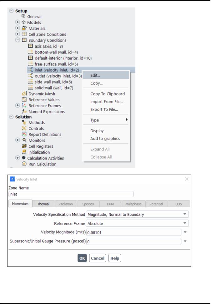
1. Set the boundary conditions for the inlet (inlet).


 Setup → Boundary Conditions → inlet
  Edit...
|
Release 2019 R1 - © ANSYS,Inc.All rights reserved.- Contains proprietary and confidential information |
682 |
of ANSYS, Inc. and its subsidiaries and affiliates. |
vk.com/club152685050 | vk.com/id446425943 |
Setup and Solution |
a.Enter 0.00101 
 for Velocity Magnitude.
b.Click the Thermal tab and enter 1300  for Temperature.
Release 2019 R1 - © ANSYS,Inc.All rights reserved.- Contains proprietary and confidential information |
|
of ANSYS, Inc. and its subsidiaries and affiliates. |
683 |
vk.com/club152685050Modeling Solidification | vk.com/id446425943
c. Click OK to close the Velocity Inlet dialog box.
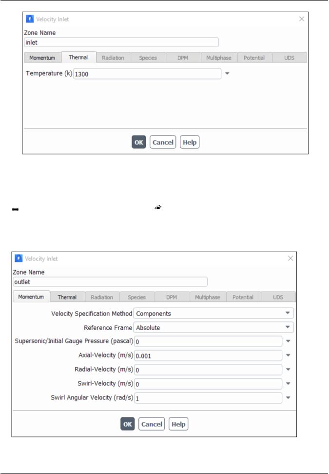
2.Set the boundary conditions for the outlet (outlet).


 Setup → Boundary Conditions → outlet
  Edit...
Here, the solid is pulled out with a specified velocity, so a velocity inlet boundary condition is used with a positive axial velocity component.
a. From the Velocity Specification Method drop-down list, select Components.
|
Release 2019 R1 - © ANSYS,Inc.All rights reserved.- Contains proprietary and confidential information |
684 |
of ANSYS, Inc. and its subsidiaries and affiliates. |

vk.com/club152685050 | vk.com/id446425943 |
Setup and Solution |
The Velocity Inlet dialog box will change to show related inputs.
b.Enter 0.001 
 for Axial-Velocity.
c.Enter 1 

 for Swirl Angular Velocity.
d.Click the Thermal tab and enter 500  for Temperature.
e. Click OK to close the Velocity Inlet dialog box.
3.Set the boundary conditions for the bottom wall (bottom-wall).


 Setup → Boundary Conditions → bottom-wall
  Edit...
a. Click the Thermal tab.
Release 2019 R1 - © ANSYS,Inc.All rights reserved.- Contains proprietary and confidential information |
|
of ANSYS, Inc. and its subsidiaries and affiliates. |
685 |

vk.com/club152685050Modeling Solidification | vk.com/id446425943
i.Select Temperature in the Thermal Conditions group box.
ii.Enter 1300  for Temperature. b. Click OK to close the Wall dialog box.
4.Set the boundary conditions for the free surface (free-surface).


 Setup → Boundary Conditions → free-surface
  Edit...
The specified shear and Marangoni stress boundary conditions are useful in modeling situations in which the shear stress (rather than the motion of the fluid) is known. A free surface condition is an example of such a situation. In this case, the convection is driven by the Marangoni stress and the shear stress is dependent on the surface tension, which is a function of temperature.
|
Release 2019 R1 - © ANSYS,Inc.All rights reserved.- Contains proprietary and confidential information |
686 |
of ANSYS, Inc. and its subsidiaries and affiliates. |
vk.com/club152685050 | vk.com/id446425943 |
Setup and Solution |
a.Select Marangoni Stress in the Shear Condition group box.
The Marangoni Stress condition allows you to specify the gradient of the surface tension with respect to temperature at a wall boundary.
b.Enter -0.00036 

 for Surface Tension Gradient.
c.Click the Thermal tab to specify the thermal conditions.
Release 2019 R1 - © ANSYS,Inc.All rights reserved.- Contains proprietary and confidential information |
|
of ANSYS, Inc. and its subsidiaries and affiliates. |
687 |

vk.com/club152685050Modeling Solidification | vk.com/id446425943
i.Select Convection from the Thermal Conditions group box.
ii.Enter 100 

 for Heat Transfer Coefficient.
iii.Enter 1500  for Free Stream Temperature. d. Click OK to close the Wall dialog box.
5.Set the boundary conditions for the side wall (side-wall).


 Setup → Boundary Conditions → side-wall
  Edit...
a. Click the Thermal tab.
|
Release 2019 R1 - © ANSYS,Inc.All rights reserved.- Contains proprietary and confidential information |
688 |
of ANSYS, Inc. and its subsidiaries and affiliates. |

vk.com/club152685050 | vk.com/id446425943 |
Setup and Solution |
i.Select Temperature from the Thermal Conditions group box.
ii.Enter 1400  for the Temperature. b. Click OK to close the Wall dialog box.
6.Set the boundary conditions for the solid wall (solid-wall).


 Setup → Boundary Conditions → solid-wall
  Edit...
Release 2019 R1 - © ANSYS,Inc.All rights reserved.- Contains proprietary and confidential information |
|
of ANSYS, Inc. and its subsidiaries and affiliates. |
689 |

vk.com/club152685050Modeling Solidification | vk.com/id446425943
a.From the Wall Motion group box, select Moving Wall.
The Wall dialog box is expanded to show additional parameters.
b.in the Motion group box, in the lower box, select Rotational.
The Wall dialog box is changed to show the rotational speed.
c.Enter 1.0 

 for Speed.
d.Click the Thermal tab to specify the thermal conditions.
|
Release 2019 R1 - © ANSYS,Inc.All rights reserved.- Contains proprietary and confidential information |
690 |
of ANSYS, Inc. and its subsidiaries and affiliates. |