vk.com/club152685050Modeling Evaporating Liquid| vk.com/id446425943Spray

5.Set the boundary conditions for the outer wall of the atomizer (outer-wall).

Setup → Boundary Conditions → outer-wall → Edit...

a.Select Specified Shear in the Shear Condition list.

b.Retain the default values for the remaining parameters.

c.Click OK to close the Wall dialog box.

16.4.7. Initial Solution Without Droplets

The airflow will first be solved and analyzed without droplets.

1.Set the solution method.

Solution → Solution → Methods...

	Release 2019 R1 - © ANSYS,Inc.All rights reserved.- Contains proprietary and confidential information
558	of ANSYS, Inc. and its subsidiaries and affiliates.

vk.com/club152685050 | vk.com/id446425943

Setup and Solution

Retain the default selections.

2.Retain the default under-relaxation factors.

Solution → Controls → Controls...

Release 2019 R1 - © ANSYS,Inc.All rights reserved.- Contains proprietary and confidential information
of ANSYS, Inc. and its subsidiaries and affiliates.	559

vk.com/club152685050Modeling Evaporating Liquid| vk.com/id446425943Spray

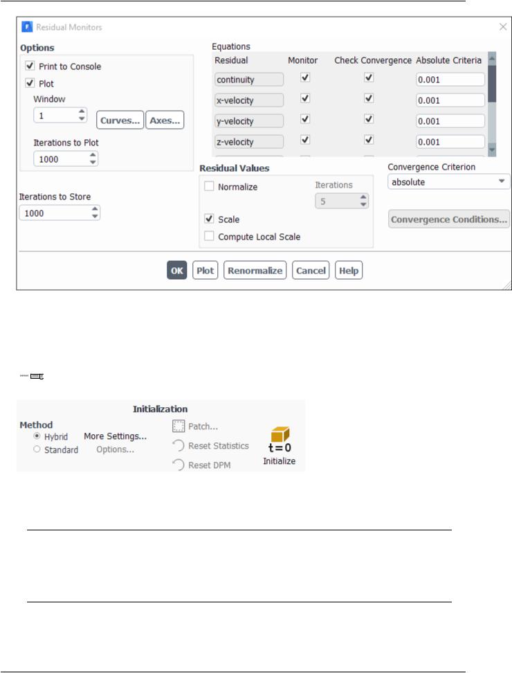
3.Enable residual plotting during the calculation.

Solution → Reports → Residuals...

	Release 2019 R1 - © ANSYS,Inc.All rights reserved.- Contains proprietary and confidential information
560	of ANSYS, Inc. and its subsidiaries and affiliates.

vk.com/club152685050 | vk.com/id446425943

Setup and Solution

a.Ensure that Plot is enabled in the Options group box.

b.Click OK to close the Residual Monitors dialog box.

4.Initialize the flow field.

Solution → Initialization

a.Retain the Method at the default of Hybrid.

b.Click Initialize to initialize the variables.

Note

For flows in complex topologies, hybrid initialization will provide better initial velocity and pressure fields than standard initialization. This will help to improve the convergence behavior of the solver.

5. Save the case file (spray1.cas.gz).

Release 2019 R1 - © ANSYS,Inc.All rights reserved.- Contains proprietary and confidential information
of ANSYS, Inc. and its subsidiaries and affiliates.	561

vk.com/club152685050Modeling Evaporating Liquid| vk.com/id446425943Spray

File → Write → Case...

6. Start the calculation by requesting 150 iterations.

Solution → Run Calculation

a.Select User Specified from the Time Step Method group box.

b.Retain 1 s for Pseudo Time Step.

c.Enter 150 for Number of Iterations.

d.Click Calculate.

Figure 16.3: Scaled Residuals

7.Save the case and data files (spray1.cas.gz and spray1.dat.gz).

File → Write → Case & Data...

Note

ANSYS Fluent will ask you to confirm that the previous case file is to be overwritten.

8.Create a clip plane to examine the flow field at the midpoint of the atomizer section.

Results → Surface → Create → Iso-Surface...

	Release 2019 R1 - © ANSYS,Inc.All rights reserved.- Contains proprietary and confidential information
562	of ANSYS, Inc. and its subsidiaries and affiliates.

vk.com/club152685050 | vk.com/id446425943

Setup and Solution

a.Enter angle=15 for New Surface Name.

b.Select Mesh... and Angular Coordinate from the Surface of Constant drop-down lists.

c.Click Compute to obtain the minimum and maximum values of the angular coordinate.

d.Enter 15 for Iso-Values.

e.Click Create to create the isosurface.

f.Close the Iso-Surface dialog box.

9.Review the current state of the solution by examining contours of velocity magnitude (Figure 16.4: Velocity Magnitude at Mid-Point of Atomizer Section (p. 565)).

Results → Graphics → Contours → Edit...

Release 2019 R1 - © ANSYS,Inc.All rights reserved.- Contains proprietary and confidential information
of ANSYS, Inc. and its subsidiaries and affiliates.	563

vk.com/club152685050Modeling Evaporating Liquid| vk.com/id446425943Spray

a.Enable Filled in the Options group box

b.Select Velocity... and Velocity Magnitude from the Contours of drop-down lists.

c.Enable Draw Mesh.

The Mesh Display dialog box will open.

i.Retain the current mesh display settings.

ii.Close the Mesh Display dialog box.

d.Select angle=15 from the Surfaces selection list.

e.Click Display and close the Contours dialog box.

f.Use the mouse to obtain the view shown in Figure 16.4: Velocity Magnitude at Mid-Point of Atomizer Section (p. 565).

	Release 2019 R1 - © ANSYS,Inc.All rights reserved.- Contains proprietary and confidential information
564	of ANSYS, Inc. and its subsidiaries and affiliates.

vk.com/club152685050 | vk.com/id446425943

Setup and Solution

Figure 16.4: Velocity Magnitude at Mid-Point of Atomizer Section

10.Modify the view to include the entire atomizer.

View → Display → Views...

a. Click the Periodic Repeats Define... button to open the Graphics Periodicity dialog box.

Release 2019 R1 - © ANSYS,Inc.All rights reserved.- Contains proprietary and confidential information
of ANSYS, Inc. and its subsidiaries and affiliates.	565

vk.com/club152685050Modeling Evaporating Liquid| vk.com/id446425943Spray

i.Select fluid from the Cell Zones selection list.

ii.Retain the selection of Rotational in the Periodic Type list.

iii.Retain the value of 12 for Number of Repeats.

iv.Click Set and close the Graphics Periodicity dialog box.

The graphics display will be updated to show the entire atomizer.

b.Click Apply and close the Views dialog box.

11.Display pathlines of the air in the swirling annular stream (Figure 16.5: Pathlines of Air in the Swirling Annular Stream (p. 568)).

Results → Graphics → Pathlines → Edit...

	Release 2019 R1 - © ANSYS,Inc.All rights reserved.- Contains proprietary and confidential information
566	of ANSYS, Inc. and its subsidiaries and affiliates.

vk.com/club152685050 | vk.com/id446425943

Setup and Solution

a.Increase the Path Skip value to 5.

b.In the Release from Surfaces filter, type s to display the surface names that begin with s and select swirling_air from the selection list.

c.Enable Draw Mesh in the Options group box.

The Mesh Display dialog box will open.

i.Retain the current mesh display settings.

ii.Close the Mesh Display dialog box.

d.Click Display and close the Pathlines dialog box.

e.Use the mouse to obtain the view shown in Figure 16.5: Pathlines of Air in the Swirling Annular Stream (p. 568).

Release 2019 R1 - © ANSYS,Inc.All rights reserved.- Contains proprietary and confidential information
of ANSYS, Inc. and its subsidiaries and affiliates.	567