vk.com/club152685050Modeling Surface Chemistry| vk.com/id446425943

File → Write → Case & Data...

15.4.10. Postprocessing the Solution Results

1.Create an iso-surface near wall-4.

Results → Surface → Create → Iso-Surface...

a. Enter z=0.07 for New Surface Name.

Note

If you want to delete or otherwise manipulate any surfaces, click Manage... to open the Surfaces dialog box.

b.Select Mesh... and Z-Coordinate from the Surface of Constant drop-down lists.

c.Click Compute.

The Min and Max fields display the z-extent of the domain.

d.Enter 0.075438 m for Iso-Values.

e.Click Create and close the Iso-Surface dialog box.

The new surface z=0.07 is added to the surfaces selection list.

2.Display contours of temperature on the plane surface created. (Figure 15.5: Temperature Contours Near wall-4 (p. 538)).

Results → Graphics → Contours → Edit...

	Release 2019 R1 - © ANSYS,Inc.All rights reserved.- Contains proprietary and confidential information
536	of ANSYS, Inc. and its subsidiaries and affiliates.

vk.com/club152685050 | vk.com/id446425943

Setup and Solution

a.Ensure that Filled is enabled in the Options group box.

b.Select Temperature... and Static Temperature from the Contours of drop-down lists.

c.Deselect wall-4 from the Surfaces selection list.

d.Select z=0.07 from the Surfaces selection list.

e.Click Display.

Release 2019 R1 - © ANSYS,Inc.All rights reserved.- Contains proprietary and confidential information
of ANSYS, Inc. and its subsidiaries and affiliates.	537

vk.com/club152685050Modeling Surface Chemistry| vk.com/id446425943

Figure 15.5: Temperature Contours Near wall-4

Figure 15.5: Temperature Contours Near wall-4 (p. 538) shows the temperature distribution across a plane just above the rotating disk. You can see that the disk has a temperature of 1023 K.

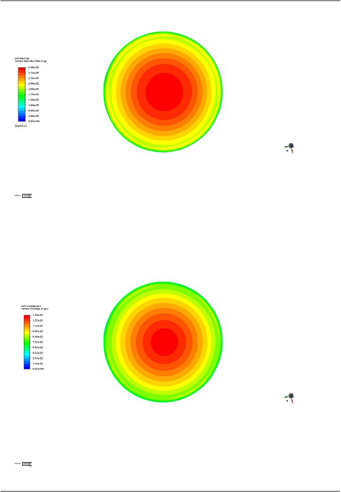
3.Display contours of surface deposition rates of ga (Figure 15.6: Contours of Surface Deposition Rate of ga (p. 539)).

Results → Graphics → Contours → Edit...

a.Select Species... and Surface Deposition Rate of ga from the Contours of drop-down lists.

b.Select wall-4 from the Surfaces selection list.

c.Deselect z=0.07 from the Surfaces selection list.

d.Click Display.

You may need to use the left mouse button to rotate the image so that you can see the contours on the top side of wall-4 where the deposition takes place.

Figure 15.6: Contours of Surface Deposition Rate of ga (p. 539) shows the gradient of surface deposition rate of ga. The maximum deposition is seen at the center of the disk.

	Release 2019 R1 - © ANSYS,Inc.All rights reserved.- Contains proprietary and confidential information
538	of ANSYS, Inc. and its subsidiaries and affiliates.

vk.com/club152685050 | vk.com/id446425943

Setup and Solution

Figure 15.6: Contours of Surface Deposition Rate of ga

4.Display contours of surface coverage of ga_s (Figure 15.7: Contours of Surface Coverage of ga_s (p. 539)).

Results → Graphics → Contours → Edit...

a.Select Species... and Surface Coverage of ga_s from the Contours of drop-down lists.

b.Retain the selection of wall-4 in the Surfaces selection list.

c.Click Display and close the Contours dialog box.

Figure 15.7: Contours of Surface Coverage of ga_s

Figure 15.7: Contours of Surface Coverage of ga_s (p. 539) shows the rate of surface coverage of the site species ga_s.

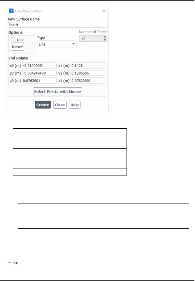
5.Create a line surface from the center of wall-4 to the edge.

Postsprocessing → Surface → Create → Line/Rake...

Release 2019 R1 - © ANSYS,Inc.All rights reserved.- Contains proprietary and confidential information
of ANSYS, Inc. and its subsidiaries and affiliates.	539

vk.com/club152685050Modeling Surface Chemistry| vk.com/id446425943

a. Enter the values for x0, x1, y0, y1, z0, and z1 as follows:

End Points	Value
x0	-0.01040954
y0	-0.004949478
z0	0.0762001
x1	0.1428
y1	0.1386585
z1	0.07620001

You can also select the points by clicking Select Points with Mouse. Then, in the graphic display, click at the center of wall-4 and at the edge using the right mouse button.

b. Click Create to accept the default name of line-9 for the New Surface Name.

Note

If you want to delete or otherwise manipulate any surfaces, click Manage... to open the Surfaces dialog box

c. Close the Line/Rake Surface dialog box.

6.Plot the surface deposition rate of Ga versus radial distance (Figure 15.8: Plot of Surface Deposition Rate of Ga (p. 542)).

Results → Plots → XY Plot → Edit...

	Release 2019 R1 - © ANSYS,Inc.All rights reserved.- Contains proprietary and confidential information
540	of ANSYS, Inc. and its subsidiaries and affiliates.

vk.com/club152685050 | vk.com/id446425943

Setup and Solution

a.Disable Node Values in the Options group box.

b.Select Species... and Surface Deposition Rate of ga from the Y Axis Function drop-down lists.

The source/sink terms due to the surface reaction are deposited in the cell adjacent to the wall cells, so it is necessary to plot the cell values and not the node values.

c.Select line-9 you just created from the Surfaces selection list.

d.Click Plot and close the Solution XY Plot dialog box.

The peak surface deposition rate occurs at the center of wall-4 (where the concentration of the mixture is highest).

Release 2019 R1 - © ANSYS,Inc.All rights reserved.- Contains proprietary and confidential information
of ANSYS, Inc. and its subsidiaries and affiliates.	541