vk.com/club152685050Modeling One-Way Fluid|-vkStructure.com/id446425943Interaction (FSI) Within Fluent

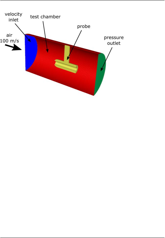
Figure 22.1: Problem Schematic

Taking advantage of the symmetry of the problem, only half of the geometry is modeled. The cylindrical test chamber is 20 cm long, with a diameter of 10 cm. Turbulent air enters the chamber at 100 m/s, flows around and through the steel probe, and exits through a pressure outlet.

22.4. Setup and Solution

The following sections describe the setup and solution steps for this tutorial:

22.4.1.Preparation

22.4.2.Structural Model

22.4.3.Materials

22.4.4.Cell Zone Conditions

22.4.5.Boundary Conditions

22.4.6.Solution

22.4.7.Postprocessing

22.4.1. Preparation

To prepare for running this tutorial:

1.Download the fsi_1way.zip file here.

2.Unzip fsi_1way.zip to your working directory.

The files probe.msh and fluid_flow.jou can be found in the folder. Note that the solid cell zone in the mesh file is appropriate for an intrinsic FSI simulation, which requires that only hexahedral and/or tetrahedral cell types are used and that a conformal mesh exists between the solid and fluid zones.

3.Use Fluent Launcher to start the 3D version of Fluent, with the Double Precision and Display Mesh After Reading options enabled. You must make sure that the Working Directory (in the General Options tab) is set to the one created when you unzipped fsi_1way.zip.

	Release 2019 R1 - © ANSYS,Inc.All rights reserved.- Contains proprietary and confidential information
750	of ANSYS, Inc. and its subsidiaries and affiliates.

vk.com/club152685050 | vk.com/id446425943

Setup and Solution

4.Read the journal file fluid_flow.jou.

File → Read → Journal...

This journal file will read the mesh file probe.msh and set up and solve a fluid flow simulation that will serve as the starting point for the structural calculations. It is not necessary to separate these calculations, but it is a advantage of one-way FSI simulation that structural calculations can be simply added to an existing fluid flow case and data file. Separating the calculations allows you to easily discern and resolve any convergence issues that are solely related to the fluid simulation.

As Fluent reads the journal file, it will report the text commands and solution progress in the console. You can also view the journal file in a text editor to see the settings used in this simulation. The final text command in the journal file will display contours of the velocity magnitude (Figure 22.2: Velocity Magnitude on the Symmetry Plane (p. 751)).

Figure 22.2: Velocity Magnitude on the Symmetry Plane

5.Save the initial case and data files as probe_fluid.cas.gz and probe_fluid.dat.gz.

File → Write → Case & Data...

Having completed the initial fluid flow simulation, the remaining steps are all concerned with setting up the structural calculations and obtaining the deformation results for the solid cell zone as a result of the flow pressure.

Release 2019 R1 - © ANSYS,Inc.All rights reserved.- Contains proprietary and confidential information
of ANSYS, Inc. and its subsidiaries and affiliates.	751

vk.com/club152685050Modeling One-Way Fluid|-vkStructure.com/id446425943Interaction (FSI) Within Fluent

22.4.2. Structural Model

1.Verify that a solid cell zone is already defined, as this is necessary to be able to enable a structural model. You can view the existing cell zones in the Outline View window.

2. Enable the linear elasticity structural model.

Setup → Models → Structure Edit...

a.Select Linear Elasticity from the Model list.

This model enables structural calculations for the solid cell zone such that the internal load is linearly proportional to the nodal displacement, and the structural stiffness matrix remains constant.

b.Click OK to close the Structural Model dialog box.

22.4.3. Materials

1. Add steel to the list of solid materials by copying it from the ANSYS Fluent materials database.

	Release 2019 R1 - © ANSYS,Inc.All rights reserved.- Contains proprietary and confidential information
752	of ANSYS, Inc. and its subsidiaries and affiliates.

vk.com/club152685050 | vk.com/id446425943

Setup and Solution

Setup → Materials → Solid → aluminum Edit...

a.Click the Fluent Database... button in the Create/Edit Materials dialog box to open the Fluent Database Materials dialog box.

i.Select solid from the Material Type drop-down list.

ii.Select steel in the Fluent Solid Materials selection list.

Scroll down the list to find steel. Selecting this item will display the default properties in the dialog box.

iii.Click Copy and close the Fluent Database Materials dialog box.

The Create/Edit Materials dialog box will now display the copied properties for steel.

Release 2019 R1 - © ANSYS,Inc.All rights reserved.- Contains proprietary and confidential information
of ANSYS, Inc. and its subsidiaries and affiliates.	753