vk.com/club152685050Modeling Species Transport| vkand.com/id446425943Gaseous Combustion

physical and thermodynamic properties are defined by your selection of the mixture material. You can alter the mixture material selection or modify the mixture material properties using the Create/Edit Materials dialog box (see Materials (p. 450)).

d.Select Eddy-Dissipation in the Turbulence-Chemistry Interaction group box.

The eddy-dissipation model computes the rate of reaction under the assumption that chemical kinetics are fast compared to the rate at which reactants are mixed by turbulent fluctuations (eddies).

e.Click OK to close the Species Model dialog box.

f.Click OK to close the Information dialog box that describes solver relaxation setting chnages.

Prior to listing the properties that are required for the models you have enabled, ANSYS Fluent will display a warning about the symmetry zone in the console. You may have to scroll up to see this warning.

Warning: It appears that symmetry zone 5 should actually be an axis (it has faces with zero area projections).

Unless you change the zone type from symmetry to axis, you may not be able to continue the solution without encountering floating point errors.

In the axisymmetric model, the boundary conditions should be such that the centerline is an axis type instead of a symmetry type. You will change the symmetry zone to an axis boundary in Boundary Conditions (p. 453).

13.5.5. Materials

In this step, you will examine the default settings for the mixture material. This tutorial uses mixture properties copied from the Fluent Database. In general, you can modify these or create your own mixture properties

for your specific problem as necessary.

1. Confirm the properties for the mixture materials.

Setup → Materials → Mixture → methane-air Edit...

The Create/Edit Materials dialog box will display the mixture material (methane-air) that was selected in the Species Model dialog box. The properties for this mixture material have been copied from the Fluent Database... and will be modified in the following steps.

	Release 2019 R1 - © ANSYS,Inc.All rights reserved.- Contains proprietary and confidential information
450	of ANSYS, Inc. and its subsidiaries and affiliates.

vk.com/club152685050 | vk.com/id446425943

Setup and Solution

a.Click the Edit... button to the right of the Mixture Species drop-down list to open the Species dialog box.

Release 2019 R1 - © ANSYS,Inc.All rights reserved.- Contains proprietary and confidential information
of ANSYS, Inc. and its subsidiaries and affiliates.	451

vk.com/club152685050Modeling Species Transport| vkand.com/id446425943Gaseous Combustion

You can add or remove species from the mixture material as necessary using the Species dialog box.

i.Retain the default selections from the Selected Species selection list.

The species that make up the methane-air mixture are predefined and require no modification.

ii.Click OK to close the Species dialog box.

b. Click the Edit... button to the right of the Reaction drop-down list to open the Reactions dialog box.

The eddy-dissipation reaction model ignores chemical kinetics (the Arrhenius rate) and uses only the parameters in the Mixing Rate group box in the Reactions dialog box. The Arrhenius Rate group box will therefore be inactive. The values for Rate Exponent and Arrhenius Rate parameters are included in the database and are employed when the alternate finite-rate/eddy-dissipation model is used.

i.Retain the default values in the Mixing Rate group box.

ii.Click OK to close the Reactions dialog box.

	Release 2019 R1 - © ANSYS,Inc.All rights reserved.- Contains proprietary and confidential information
452	of ANSYS, Inc. and its subsidiaries and affiliates.

vk.com/club152685050 | vk.com/id446425943

Setup and Solution

c.Retain the selection of incompressible-ideal-gas from the Density drop-down list.

d.Retain the selection of mixing-law from the Cp (Specific Heat) drop-down list.

e.Retain the default values for Thermal Conductivity, Viscosity, and Mass Diffusivity.

f.Click Change/Create to accept the material property settings.

g.Close the Create/Edit Materials dialog box.

The calculation will be performed assuming that all properties except density and specific heat are constant. The use of constant transport properties (viscosity, thermal conductivity, and mass diffusivity coefficients) is acceptable because the flow is fully turbulent. The molecular transport properties will play a minor role compared to turbulent transport.

13.5.6. Boundary Conditions

1. Convert the symmetry zone to the axis type.

Setup → Boundary Conditions → symmetry-5 Typeaxis

The symmetry zone must be converted to an axis to prevent numerical difficulties where the radius reduces to zero.

2. Set the boundary conditions for the air inlet (velocity-inlet-8).

Setup → Boundary Conditions → velocity-inlet-8 Edit...

To determine the zone for the air inlet, display the mesh without the fluid zone to see the boundaries. Use the right mouse button to probe the air inlet. ANSYS Fluent will report the zone name (velocity-inlet- 8) in the console.

Release 2019 R1 - © ANSYS,Inc.All rights reserved.- Contains proprietary and confidential information
of ANSYS, Inc. and its subsidiaries and affiliates.	453

vk.com/club152685050Modeling Species Transport| vkand.com/id446425943Gaseous Combustion

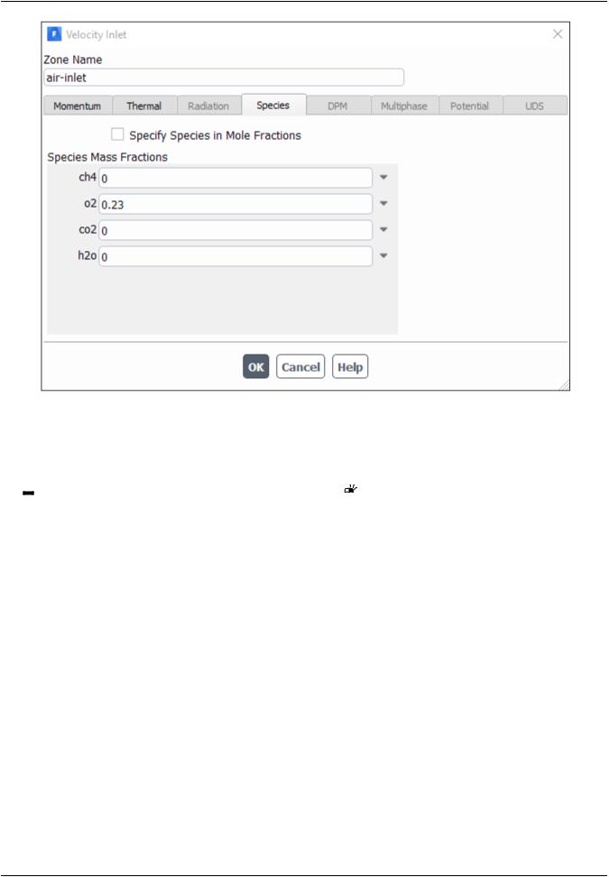
a.Enter air-inlet for Zone Name.

This name is more descriptive for the zone than velocity-inlet-8.

b.Enter 0.5 for Velocity Magnitude.

c.Select Intensity and Hydraulic Diameter from the Specification Method drop-down list in the Turbulence group box.

d.Enter 10 for Turbulent Intensity.

e.Enter 0.44 for Hydraulic Diameter.

f.Click the Thermal tab and retain the default value of 300 for Temperature.

g.Click the Species tab and enter 0.23 for o2 in the Species Mass Fractions group box.

	Release 2019 R1 - © ANSYS,Inc.All rights reserved.- Contains proprietary and confidential information
454	of ANSYS, Inc. and its subsidiaries and affiliates.

vk.com/club152685050 | vk.com/id446425943

Setup and Solution

h. Click OK to close the Velocity Inlet dialog box.

3.Set the boundary conditions for the fuel inlet (velocity-inlet-6).

Setup → Boundary Conditions → velocity-inlet-6 Edit...

Release 2019 R1 - © ANSYS,Inc.All rights reserved.- Contains proprietary and confidential information
of ANSYS, Inc. and its subsidiaries and affiliates.	455

vk.com/club152685050Modeling Species Transport| vkand.com/id446425943Gaseous Combustion

a.Enter fuel-inlet for Zone Name.

This name is more descriptive for the zone than velocity-inlet-6.

b.Enter 80 for the Velocity Magnitude.

c.Select Intensity and Hydraulic Diameter from the Specification Method drop-down list in the Turbulence group box.

d.Enter 10 for Turbulent Intensity.

e.Enter 0.01 for Hydraulic Diameter.

f.Click the Thermal tab and retain the default value of 300 for Temperature.

g.Click the Species tab and enter 1 for ch4 in the Species Mass Fractions group box.

h.Click OK to close the Velocity Inlet dialog box.

4.Set the boundary conditions for the exit boundary (pressure-outlet-9).

Setup → Boundary Conditions → pressure-outlet-9 Edit...

	Release 2019 R1 - © ANSYS,Inc.All rights reserved.- Contains proprietary and confidential information
456	of ANSYS, Inc. and its subsidiaries and affiliates.

vk.com/club152685050 | vk.com/id446425943

Setup and Solution

a.Retain the default value of 0 for Gauge Pressure.

b.Select Intensity and Hydraulic Diameter from the Specification Method drop-down list in the Turbulence group box.

c.Enter 10 for Backflow Turbulent Intensity.

d.Enter 0.45 for Backflow Hydraulic Diameter.

e.Click the Thermal tab and retain the default value of 300 for Backflow Total Temperature.

f.Click the Species tab and enter 0.23 for o2 in the Species Mass Fractions group box.

g.Click OK to close the Pressure Outlet dialog box.

The Backflow values in the Pressure Outlet dialog box are utilized only when backflow occurs at the pressure outlet. Always assign reasonable values because backflow may occur during intermediate iterations and could affect the solution stability.

5. Set the boundary conditions for the outer wall (wall-7).

Setup → Boundary Conditions → wall-7 Edit...

Release 2019 R1 - © ANSYS,Inc.All rights reserved.- Contains proprietary and confidential information
of ANSYS, Inc. and its subsidiaries and affiliates.	457

vk.com/club152685050Modeling Species Transport| vkand.com/id446425943Gaseous Combustion

Use the mouse-probe method described for the air inlet to determine the zone corresponding to the outer wall.

a.Enter outer-wall for Zone Name.

This name is more descriptive for the zone than wall-7.

b.Click the Thermal tab.

i.Select Temperature in the Thermal Conditions list.

ii.Retain the default value of 300 for Temperature.

c.Click OK to close the Wall dialog box.

6.Set the boundary conditions for the fuel inlet nozzle (wall-2).

Setup → Boundary Conditions → wall-2 Edit...

	Release 2019 R1 - © ANSYS,Inc.All rights reserved.- Contains proprietary and confidential information
458	of ANSYS, Inc. and its subsidiaries and affiliates.