vk.com/club152685050Fluid Flow and Heat Transfer| vk.incom/id446425943a Mixing Elbow

2.4.3. Reading the Mesh

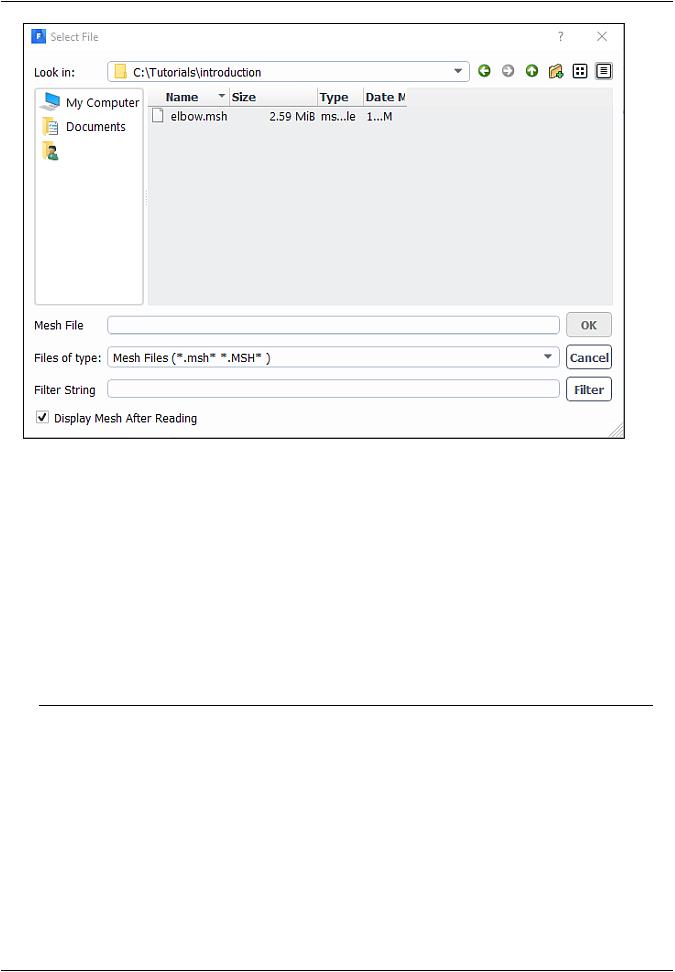
1.Read the mesh file elbow.msh.

Click the File ribbon tab, then click Read and Mesh... in the menus that open in order to open the

Select File dialog box.

File → Read → Mesh...

	Release 2019 R1 - © ANSYS,Inc.All rights reserved.- Contains proprietary and confidential information
40	of ANSYS, Inc. and its subsidiaries and affiliates.

vk.com/club152685050 | vk.com/id446425943

Setup and Solution

a.Select the mesh file by clicking elbow.msh in the introduction folder created when you unzipped the original file.

b.Enable the Display Mesh After Reading in the Select File panel.

c.Click OK to read the file and close the Select File dialog box.

As the mesh file is read by ANSYS Fluent, messages will appear in the console reporting the progress of the conversion. ANSYS Fluent will report that 13,852 hexahedral fluid cells have been read, along with a number of boundary faces with different zone identifiers.

After having completed reading mesh, ANSYS Fluent displays the mesh in the graphics window.

Extra

You can use the mouse to probe for mesh information in the graphics window. If you click the right mouse button with the pointer on any node in the mesh, information about the associated zone will be displayed in the console, including the name of the zone.

Alternatively, you can click the probe button () in the graphics toolbar and click the left mouse button on any node. This feature is especially useful when you have several zones of the same type and you want to distinguish between them quickly.

Release 2019 R1 - © ANSYS,Inc.All rights reserved.- Contains proprietary and confidential information
of ANSYS, Inc. and its subsidiaries and affiliates.	41

vk.com/club152685050Fluid Flow and Heat Transfer| vk.incom/id446425943a Mixing Elbow

For this 3D problem, you can make it easier to probe particular nodes by changing the view. The following table describes how to manipulate objects in the graphics window:

Table 2.1: View Manipulation Instructions

Action Using Graphics Toolbar Buttons and the Mouse

Rotate view (vertical, horizontal)

After clicking the Rotate View icon, , press and hold the left mouse button and drag the mouse. Dragging side to side rotates the view about the vertical axis, and dragging up and down rotates the view about the horizontal axis.

Translate or

pan view After clicking the Pan icon, , press and hold the left mouse button and drag the object with the mouse until the view is satisfactory.

Zoom in and

out of view After clicking the Zoom In/Out icon, , press and hold the left mouse button and drag the mouse up and down to zoom in and out of the view.

Zoom to selected area

After clicking the Zoom to Area icon, , press and hold the left mouse button and drag the mouse diagonally to the right. This action will cause a rectangle to appear in the display. When you release the mouse button, a new view will be displayed that consists entirely of the contents of the rectangle. Note that to zoom in, you must drag the mouse to the right, and to zoom out, you must drag the mouse to the left.

Clicking the Fit to Window icon, , will cause the object to fit exactly and be centered in the window.

After you have clicked a button in the graphics toolbar, you can return to the default mouse button settings by clicking .

To judge the scale of your 3D geometry, you can click the Orthographic Projection icon,

. This will display the length scale ruler near the bottom of the graphics window.

Note that you can change the default mouse button actions in the View tab (in the Mouse group box). For more information, see the Fluent User's Guide.

2.Manipulate the mesh display using the axis triad to obtain a front view as shown in Figure 2.2: The Hexahedral Mesh for the Mixing Elbow (p. 43).

a.Click the z-axis.

b.Clicking the Fit to Window icon, , will cause the object to fit exactly and be centered in the window.

	Release 2019 R1 - © ANSYS,Inc.All rights reserved.- Contains proprietary and confidential information
42	of ANSYS, Inc. and its subsidiaries and affiliates.

vk.com/club152685050 | vk.com/id446425943

Setup and Solution

c. Figure 2.2: The Hexahedral Mesh for the Mixing Elbow

Extra

You can also change the orientation of the objects in the graphics window using the

axis triad as follows:

•To orient the model in the positive/negative direction, click an axis/semi-sphere.

•To orient the model in the negative/positive direction, right-click an axis/semi-sphere.

•To set the isometric view, click the cyan iso-ball.

•To perform in-plane clockwise or counterclockwise 90° rotations, click the white rotational arrows .

•To perform free rotations in any direction, click and hold—in the vicinity of the triad—and use the mouse. Release the left mouse button to stop rotating.

2.4.4.Setting Up Domain

In this step, you will perform the mesh-related activities using the Domain ribbon tab (Mesh group box).

Release 2019 R1 - © ANSYS,Inc.All rights reserved.- Contains proprietary and confidential information
of ANSYS, Inc. and its subsidiaries and affiliates.	43

vk.com/club152685050Fluid Flow and Heat Transfer| vk.incom/id446425943a Mixing Elbow

1.Check the mesh.

Domain → Mesh → Check → Perform Mesh Check

ANSYS Fluent will report the results of the mesh check in the console.

Domain Extents:

x-coordinate: min (m) = -8.000000e+00, max (m) = 8.000000e+00 y-coordinate: min (m) = -9.134634e+00, max (m) = 8.000000e+00 z-coordinate: min (m) = 0.000000e+00, max (m) = 2.000000e+00

Volume statistics:

minimum volume (m3): 5.098304e-04 maximum volume (m3): 2.330736e-02 total volume (m3): 1.607154e+02

Face area statistics:

minimum face area (m2): 4.865882e-03 maximum face area (m2): 1.017924e-01

Checking mesh....................................

Done.

The mesh check will list the minimum and maximum x, y, and z values from the mesh in the default SI unit of meters. It will also report a number of other mesh features that are checked. Any errors in the mesh will be reported at this time. Ensure that the minimum volume is not negative, since ANSYS Fluent cannot begin a calculation when this is the case.

Note

The minimum and maximum values may vary slightly when running on different platforms.

2.Scale the mesh.

Domain → Mesh → Scale...

	Release 2019 R1 - © ANSYS,Inc.All rights reserved.- Contains proprietary and confidential information
44	of ANSYS, Inc. and its subsidiaries and affiliates.

vk.com/club152685050 | vk.com/id446425943

Setup and Solution

a.Ensure that Convert Units is selected in the Scaling group box.

b.From the Mesh Was Created In drop-down list, select in by first clicking the down-arrow button and then clicking the in item from the list that appears.

c.Click Scale to scale the mesh.

Warning

Be sure to click the Scale button only once.

Domain Extents will continue to be reported in the default SI unit of meters.

d.Select in from the View Length Unit In drop-down list to set inches as the working unit for length.

e.Confirm that the domain extents are as shown in the previous dialog box.

f.Close the Scale Mesh dialog box.

The mesh is now sized correctly and the working unit for length has been set to inches.

Note

Because the default SI units will be used for everything except length, there is no need to change any other units in this problem. The choice of inches for the unit of length has been made by the actions you have just taken. If you want a different working unit for length, other than inches (for example, millimeters), click Units... in the Domain ribbon tab (Mesh group box) and make the appropriate change in the Set Units dialog box.

Release 2019 R1 - © ANSYS,Inc.All rights reserved.- Contains proprietary and confidential information
of ANSYS, Inc. and its subsidiaries and affiliates.	45