vk.com/club152685050 | vk.com/id446425943

Setup and Solution

i.Select Temperature from the Thermal Conditions selection list.

ii.Enter 500 for Temperature.

e. Click OK to close the Wall dialog box.

20.4.8. Solution: Steady Conduction

In this step, you will specify the discretization schemes to be used and temporarily disable the calculation of the flow and swirl velocity equations, so that only conduction is calculated. This steady-state solution will be used as the initial condition for the time-dependent fluid flow and heat transfer calculation.

1.Set the solution parameters.

Solution → Solution → Methods...

Release 2019 R1 - © ANSYS,Inc.All rights reserved.- Contains proprietary and confidential information
of ANSYS, Inc. and its subsidiaries and affiliates.	691

vk.com/club152685050Modeling Solidification | vk.com/id446425943

a.Select Coupled from the Scheme drop-down list in the Pressure-Velocity Coupling group box.

b.Select PRESTO! from the Pressure drop-down list in the Spatial Discretization group box.

The PRESTO! scheme is well suited for rotating flows with steep pressure gradients.

c.Retain the default selection of Second Order Upwind from the Momentum, Swirl Velocity, and Energy drop-down lists.

d.Enable Pseudo Transient.

The Pseudo Transient option enables the pseudo transient algorithm in the coupled pressure-based solver. This algorithm effectively adds an unsteady term to the solution equations in order to improve stability and convergence behavior. Use of this option is recommended for general fluid flow problems.

2. Enable the calculation for energy.

	Release 2019 R1 - © ANSYS,Inc.All rights reserved.- Contains proprietary and confidential information
692	of ANSYS, Inc. and its subsidiaries and affiliates.

vk.com/club152685050 | vk.com/id446425943

Setup and Solution

Solution → Controls → Equations...

a.Deselect Flow and Swirl Velocity from the Equations selection list to disable the calculation of flow and swirl velocity equations.

b.Click OK to close the Equations dialog box.

3.Confirm the Relaxation Factors.

Solution → Controls → Controls...

Release 2019 R1 - © ANSYS,Inc.All rights reserved.- Contains proprietary and confidential information
of ANSYS, Inc. and its subsidiaries and affiliates.	693

vk.com/club152685050Modeling Solidification | vk.com/id446425943

Retain the default values.

4.Enable the plotting of residuals during the calculation.

Solution → Reports → Residuals...

	Release 2019 R1 - © ANSYS,Inc.All rights reserved.- Contains proprietary and confidential information
694	of ANSYS, Inc. and its subsidiaries and affiliates.

vk.com/club152685050 | vk.com/id446425943

Setup and Solution

a.Ensure Plot is enabled in the Options group box.

b.Click OK to accept the remaining default settings and close the Residual Monitors dialog box.

5.Initialize the solution.

Solution → Initialization

a.Retain the Method at the default of Hybrid in the Initialization group.

For flows in complex topologies, hybrid initialization will provide better initial velocity and pressure field than standard initialization. This in general will help in improving the convergence behavior of the solver.

b.Click Initialize.

6.Define a custom field function for the swirl pull velocity.

Parameters & Customization → Custom Field Functions New...

In this step, you will define a field function to be used to patch a variable value for the swirl pull velocity in the next step. The swirl pull velocity is equal to , where is the angular velocity, and is the radial coordinate. Since = 1 rad/s, you can simplify the equation to simply . In this example, the value of is included for demonstration purposes.

Release 2019 R1 - © ANSYS,Inc.All rights reserved.- Contains proprietary and confidential information
of ANSYS, Inc. and its subsidiaries and affiliates.	695

vk.com/club152685050Modeling Solidification | vk.com/id446425943

a.From the Field Functions drop-down lists, select Mesh... and Radial Coordinate.

b.Click the Select button to add radial-coordinate in the Definition field.

If you make a mistake, click the DEL button on the calculator pad to delete the last item you added to the function definition.

c.Click the button on the calculator pad.

d.Click the 1 button.

e.Enter omegar for New Function Name.

f.Click Define.

The omegar item appears under the Parameters & Customisation/Parameters tree branch.

Note

To check the function definition or delete the custom field function, click Manage....

Then in the Field Function Definitions dialog box, from the Field Functions selection list, select omegar to view the function definition.

g. Close the Custom Field Function Calculator dialog box.

7.Patch the pull velocities.

Solution → Initialization → Patch...

As noted earlier, you will patch values for the pull velocities, rather than having ANSYS Fluent compute them. Since the radial pull velocity is zero, you will patch just the axial and swirl pull velocities.

	Release 2019 R1 - © ANSYS,Inc.All rights reserved.- Contains proprietary and confidential information
696	of ANSYS, Inc. and its subsidiaries and affiliates.

vk.com/club152685050 | vk.com/id446425943

Setup and Solution

a.From the Variable selection list, select Axial Pull Velocity.

b.Enter 0.001 for Value.

c.From the Zones to Patch selection list, select fluid.

d.Click Patch.

You have just patched the axial pull velocity. Next you will patch the swirl pull velocity.

e.From the Variable selection list, select Swirl Pull Velocity.

Scroll down the list to find Swirl Pull Velocity.

f.Enable the Use Field Function option.

g.Select omegar from the Field Function selection list.

h.Ensure that fluid is selected from the Zones to Patch selection list.

i.Click Patch and close the Patch dialog box.

Release 2019 R1 - © ANSYS,Inc.All rights reserved.- Contains proprietary and confidential information
of ANSYS, Inc. and its subsidiaries and affiliates.	697

vk.com/club152685050Modeling Solidification | vk.com/id446425943

8.Save the initial case and data files (solid0.cas.gz and solid0.dat.gz).

File → Write → Case & Data...

9.Start the calculation by requesting 20 iterations.

Solution → Run Calculation → Advanced...

a.In the Run Calculation task page, select User Specified for the Time Step Method in both the Fluid Time Scale and the Solid Time Scale group boxes.

	Release 2019 R1 - © ANSYS,Inc.All rights reserved.- Contains proprietary and confidential information
698	of ANSYS, Inc. and its subsidiaries and affiliates.

vk.com/club152685050 | vk.com/id446425943

Setup and Solution

b.Retain the default values of 1 and 1000 for the Pseudo Time Step (s) in the Fluid Time Scale and the Solid Time Scale group boxes, respectively.

c.Enter 20 for Number of Iterations.

d.Click Calculate.

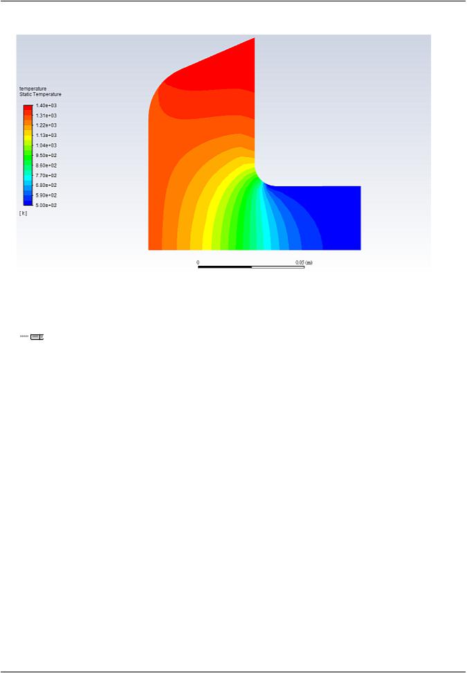
10.Create and display the definition of filled temperature contours (Figure 20.3: Contours of Temperature for the Steady Conduction Solution (p. 700)).

Results → Graphics → Contours → New...

a.Enter temperature for Contour Name.

b.Enable the Filled option.

c.Enable the Banded option.

d.Select Temperature... and Static Temperature from the Contours of drop-down lists.

e.Click Save/Display (Figure 20.3: Contours of Temperature for the Steady Conduction Solution (p. 700)). The temperature contour definition appear under the Results/Graphics/Contours tree branch.

Release 2019 R1 - © ANSYS,Inc.All rights reserved.- Contains proprietary and confidential information
of ANSYS, Inc. and its subsidiaries and affiliates.	699

vk.com/club152685050Modeling Solidification | vk.com/id446425943

Figure 20.3: Contours of Temperature for the Steady Conduction Solution

11.Display filled contours of temperature to determine the thickness of mushy zone.

Results → Graphics → Contours → Edit...

	Release 2019 R1 - © ANSYS,Inc.All rights reserved.- Contains proprietary and confidential information
700	of ANSYS, Inc. and its subsidiaries and affiliates.

vk.com/club152685050 | vk.com/id446425943

Setup and Solution

a.Disable Auto Range in the Options group box.

The Clip to Range option is automatically enabled.

b.Enter 1100 for Min and 1200 for Max.

c.Click Display (See Figure 20.4: Contours of Temperature (Mushy Zone) for the Steady Conduction Solution (p. 702)) and close the Contours dialog box.

Release 2019 R1 - © ANSYS,Inc.All rights reserved.- Contains proprietary and confidential information
of ANSYS, Inc. and its subsidiaries and affiliates.	701

vk.com/club152685050Modeling Solidification | vk.com/id446425943

Figure 20.4: Contours of Temperature (Mushy Zone) for the Steady Conduction Solution

12. Save the case and data files for the steady conduction solution (solid.cas.gz and solid.dat.gz).

File → Write → Case & Data...

20.4.9. Solution:Transient Flow and Heat Transfer

In this step, you will turn on time dependence and include the flow and swirl velocity equations in the calculation. You will then solve the transient problem using the steady conduction solution as the initial condition.

1.Enable a time-dependent solution by selecting Transient from the Time list.

Setup → General

	Release 2019 R1 - © ANSYS,Inc.All rights reserved.- Contains proprietary and confidential information
702	of ANSYS, Inc. and its subsidiaries and affiliates.

vk.com/club152685050 | vk.com/id446425943

Setup and Solution

2.Set the solution parameters.

Solution → Solution → Methods...

Release 2019 R1 - © ANSYS,Inc.All rights reserved.- Contains proprietary and confidential information
of ANSYS, Inc. and its subsidiaries and affiliates.	703

vk.com/club152685050Modeling Solidification | vk.com/id446425943

a.Retain the default selection of First Order Implicit from the Transient Formulation drop-down list.

b.Ensure that PRESTO! is selected from the Pressure drop-down list in the Spatial Discretization group box.

3.Enable calculations for flow and swirl velocity.

Solution → Controls → Equations...

	Release 2019 R1 - © ANSYS,Inc.All rights reserved.- Contains proprietary and confidential information
704	of ANSYS, Inc. and its subsidiaries and affiliates.

vk.com/club152685050 | vk.com/id446425943

Setup and Solution

a.Select Flow and Swirl Velocity and ensure that Energy is selected from the Equations selection list.

Now all three items in the Equations selection list will be selected.

b.Click OK to close the Equations dialog box.

4.Set the Under-Relaxation Factors.

Solution → Controls → Controls...

Release 2019 R1 - © ANSYS,Inc.All rights reserved.- Contains proprietary and confidential information
of ANSYS, Inc. and its subsidiaries and affiliates.	705

vk.com/club152685050Modeling Solidification | vk.com/id446425943

a.Enter 0.1 for Liquid Fraction Update.

b.Retain the default values for other Under-Relaxation Factors.

5.Save the initial case and data files (solid01.cas.gz and solid01.dat.gz).

File → Write → Case & Data...

6.Run the calculation for 2 time steps.

Solution → Run Calculation → Advanced...

	Release 2019 R1 - © ANSYS,Inc.All rights reserved.- Contains proprietary and confidential information
706	of ANSYS, Inc. and its subsidiaries and affiliates.

vk.com/club152685050 | vk.com/id446425943

Setup and Solution

a.Enter 0.1 s for Time Step Size.

b.Set the Number of Time Steps to 2.

c.Retain the default value of 20 for Max Iterations/Time Step.

d.Click Calculate.

7.Display filled contours of the temperature after 0.2 seconds using the temperature contours definition that you created earlier.

Results → Graphics → Contours → temperature Display

Release 2019 R1 - © ANSYS,Inc.All rights reserved.- Contains proprietary and confidential information
of ANSYS, Inc. and its subsidiaries and affiliates.	707

vk.com/club152685050Modeling Solidification | vk.com/id446425943

Figure 20.5: Contours of Temperature at t=0.2 s

8.Create and display the definition of stream function contours (Figure 20.6: Contours of Stream Function at t=0.2 s (p. 709)).

Results → Graphics → Contours → New...

a.Enter stream-function for Contour Name.

b.Disable Filled in the Options group box.

c.Disable Global Range.

d.Ensure that the Auto Range is enabled.

e.Select Velocity... and Stream Function from the Contours of drop-down lists.

f.Click Save/Display.

The stream-function contour definition appear under the Results/Graphics/Contours tree branch.

	Release 2019 R1 - © ANSYS,Inc.All rights reserved.- Contains proprietary and confidential information
708	of ANSYS, Inc. and its subsidiaries and affiliates.

vk.com/club152685050 | vk.com/id446425943

Setup and Solution

Figure 20.6: Contours of Stream Function at t=0.2 s

As shown in Figure 20.6: Contours of Stream Function at t=0.2 s (p. 709), the liquid is beginning to circulate in a large eddy, driven by natural convection and Marangoni convection on the free surface.

9.Create and display the definition of liquid fraction contours by modifying the stream-function contour definition (Figure 20.7: Contours of Liquid Fraction at t=0.2 s (p. 710)).

Results → Graphics → Contours → New...

a.Enter liquid-fraction for Contour Name.

b.Enable Filled in the Options group box.

c.Enable Auto Range in the Options group box.

d.Select Solidification/Melting... and Liquid Fraction from the Contours of drop-down lists.

e.Click Save/Display and close the Contours dialog box.

Release 2019 R1 - © ANSYS,Inc.All rights reserved.- Contains proprietary and confidential information
of ANSYS, Inc. and its subsidiaries and affiliates.	709

vk.com/club152685050Modeling Solidification | vk.com/id446425943

Figure 20.7: Contours of Liquid Fraction at t=0.2 s

The liquid fraction contours show the current position of the melt front. Note that in Figure 20.7: Contours of Liquid Fraction at t=0.2 s (p. 710), the mushy zone divides the liquid and solid regions roughly in half.

10.Continue the calculation for 48 additional time steps.

Solution → Run Calculation → Advanced...

a.Enter 48 for Number of Time Steps.

b.Click Calculate.

After a total of 50 time steps have been completed, the elapsed time will be 5 seconds.

11.Display filled contours of the temperature after 5 seconds using the contour definition created earlier (Figure 20.8: Contours of Temperature at t=5 s (p. 711)).

Results → Graphics → Contours → temperature Display

	Release 2019 R1 - © ANSYS,Inc.All rights reserved.- Contains proprietary and confidential information
710	of ANSYS, Inc. and its subsidiaries and affiliates.

vk.com/club152685050 | vk.com/id446425943

Setup and Solution

Figure 20.8: Contours of Temperature at t=5 s

As shown in Figure 20.8: Contours of Temperature at t=5 s (p. 711), the temperature contours are fairly uniform through the melt front and solid material. The distortion of the temperature field due to the recirculating liquid is also clearly evident.

In a continuous casting process, it is important to pull out the solidified material at the proper time. If the material is pulled out too soon, it will not have solidified (that is, it will still be in a mushy state). If it is pulled out too late, it solidifies in the casting pool and cannot be pulled out in the required shape. The optimal rate of pull can be determined from the contours of liquidus temperature and solidus temperature.

12. Display contours of stream function (Figure 20.9: Contours of Stream Function at t=5 s (p. 712)).

Results → Graphics → Contours → stream-function Display

As shown in Figure 20.9: Contours of Stream Function at t=5 s (p. 712), the flow has developed more fully by 5 seconds, as compared with Figure 20.6: Contours of Stream Function at t=0.2 s (p. 709) after 0.2 seconds. The main eddy, driven by natural convection and Marangoni stress, dominates the flow.

Release 2019 R1 - © ANSYS,Inc.All rights reserved.- Contains proprietary and confidential information
of ANSYS, Inc. and its subsidiaries and affiliates.	711

vk.com/club152685050Modeling Solidification | vk.com/id446425943

Figure 20.9: Contours of Stream Function at t=5 s

To examine the position of the melt front and the extent of the mushy zone, you will plot the contours of liquid fraction.

13. Display filled contours of liquid fraction (Figure 20.10: Contours of Liquid Fraction at t=5 s (p. 713)).

Results → Graphics → Contours → liquid-fraction

Display

The introduction of liquid material at the left of the domain is balanced by the pulling of the solidified material from the right. After 5 seconds, the equilibrium position of the melt front is beginning to be established (Figure 20.10: Contours of Liquid Fraction at t=5 s (p. 713)).

	Release 2019 R1 - © ANSYS,Inc.All rights reserved.- Contains proprietary and confidential information
712	of ANSYS, Inc. and its subsidiaries and affiliates.