


vk.com/club152685050Fluid Flow and Heat Transfer| vk.incom/id446425943a Mixing Elbow
10.Examine the mass flux report for convergence using the Results ribbon tab.

 Results → Reports → Fluxes...
a.Ensure that Mass Flow Rate is selected from the Options list.
b.Select pressure-outlet-7, velocity-inlet-5, and velocity-inlet-6 from the Boundaries selection list.
c.Click Compute.
The individual and net results of the computation will be displayed in the Results and Net Results boxes, respectively, in the Flux Reports dialog box, as well as in the console.
The sum of the flux for the inlets should be very close to the sum of the flux for the outlets. The net results show that the imbalance in this case is well below the 0.2% criterion suggested previously.
d.Close the Flux Reports dialog box.
11.Save the data file (elbow1.dat.gz).

 File → Write → Data...
In later steps of this tutorial you will save additional case and data files with different suffixes.
2.4.7. Displaying the Preliminary Solution
In the steps that follow, you will visualize various aspects of the flow for the preliminary solution using the Results ribbon tab.
1.Display filled contours of velocity magnitude on the symmetry plane (Figure 2.5: Predicted Velocity Distribution after the Initial Calculation (p. 70)).
 Results → Graphics → Contours → Edit...
|
Release 2019 R1 - © ANSYS,Inc.All rights reserved.- Contains proprietary and confidential information |
68 |
of ANSYS, Inc. and its subsidiaries and affiliates. |

vk.com/club152685050 | vk.com/id446425943 |
Setup and Solution |
a.Enable Filled in the Options group box.
b.Ensure that Node Values is enabled in the Options group box.
c.Select Velocity... and Velocity Magnitude from the Contours of drop-down lists.
d.Select symmetry from the Surfaces selection list.
e.Click Display to display the contours in the active graphics window. Clicking the Fit to Window icon ( ) will cause the object to fit exactly and be centered in the window.
Note
If you cannot see the velocity contour display, select the appropriate tab in the graphics window.
f.Close the Contours dialog box.

 View → Display
Release 2019 R1 - © ANSYS,Inc.All rights reserved.- Contains proprietary and confidential information |
|
of ANSYS, Inc. and its subsidiaries and affiliates. |
69 |

vk.com/club152685050Fluid Flow and Heat Transfer| vk.incom/id446425943a Mixing Elbow
Disable the Headlight and Lighting options.
Figure 2.5: Predicted Velocity Distribution after the Initial Calculation
Extra
When you probe a point in the displayed domain with the right mouse button or the probe tool, the level of the corresponding contour is highlighted in the colormap in the graphics window, and is also reported in the console.
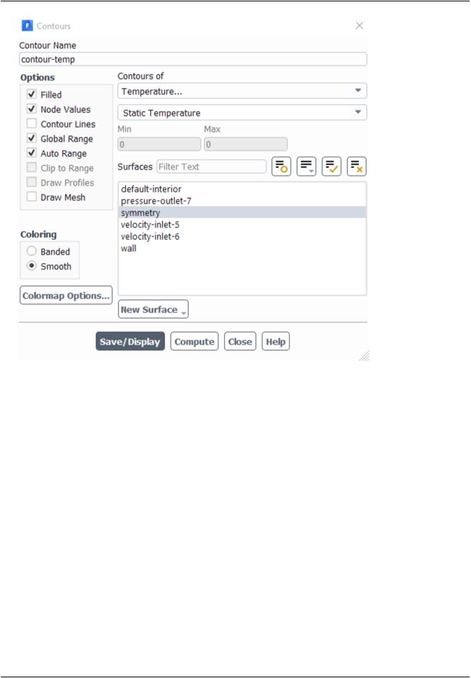
2.Create and display a definition for temperature contours on the symmetry plane (Figure 2.6: Predicted Temperature Distribution after the Initial Calculation (p. 72)).
 Results → Graphics → Contours → New...
You can create contour definitions and save them for later use.
|
Release 2019 R1 - © ANSYS,Inc.All rights reserved.- Contains proprietary and confidential information |
70 |
of ANSYS, Inc. and its subsidiaries and affiliates. |
vk.com/club152685050 | vk.com/id446425943 |
Setup and Solution |
a.Enter contour-temp for Contour Name.
b.Select Temperature... and Static Temperature from the Contours of drop-down lists.
c.Click Save/Display and close the Contours dialog box.
The new contour-temp definition appears under the Results/Graphics/Contours tree branch. To edit your contour definition, right-click it and select Edit... from the menu that opens.
Release 2019 R1 - © ANSYS,Inc.All rights reserved.- Contains proprietary and confidential information |
|
of ANSYS, Inc. and its subsidiaries and affiliates. |
71 |

vk.com/club152685050Fluid Flow and Heat Transfer| vk.incom/id446425943a Mixing Elbow
Figure 2.6: Predicted Temperature Distribution after the Initial Calculation
3.Display velocity vectors on the symmetry plane (Figure 2.9: Magnified View of Resized Velocity Vectors (p. 74)).
 Results → Graphics → Vectors → Edit...
|
Release 2019 R1 - © ANSYS,Inc.All rights reserved.- Contains proprietary and confidential information |
72 |
of ANSYS, Inc. and its subsidiaries and affiliates. |

vk.com/club152685050 | vk.com/id446425943 |
Setup and Solution |
a.Select symmetry from the Surfaces selection list.
b.Click Display to plot the velocity vectors.
Figure 2.7: Velocity Vectors Colored by Velocity Magnitude
The Auto Scale option is enabled by default in the Options group box. This scaling sometimes creates vectors that are too small or too large in the majority of the domain. You can improve the clarity by adjusting the Scale and Skip settings, thereby changing the size and number of the vectors when they are displayed.
c.Enter 4 for Scale.
d.Set Skip to 2.
e.Click Display again to redisplay the vectors.
Release 2019 R1 - © ANSYS,Inc.All rights reserved.- Contains proprietary and confidential information |
|
of ANSYS, Inc. and its subsidiaries and affiliates. |
73 |
vk.com/club152685050Fluid Flow and Heat Transfer| vk.incom/id446425943a Mixing Elbow
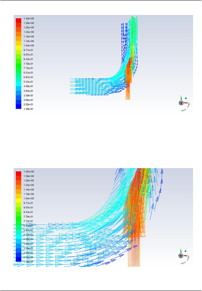
Figure 2.8: Resized Velocity Vectors
f.Close the Vectors dialog box.
g.Zoom in on the vectors in the display.
To manipulate the image, refer to Table 2.1: View Manipulation Instructions (p. 42). The image will
be redisplayed at a higher magnification (Figure 2.9: Magnified View of Resized Velocity Vectors (p. 74)).
Figure 2.9: Magnified View of Resized Velocity Vectors
h. Zoom out to the original view.
|
Release 2019 R1 - © ANSYS,Inc.All rights reserved.- Contains proprietary and confidential information |
74 |
of ANSYS, Inc. and its subsidiaries and affiliates. |

vk.com/club152685050 | vk.com/id446425943 |
Setup and Solution |
Clicking the Fit to Window icon,  , will cause the object to fit exactly and be centered in the window.
4.Create a line at the centerline of the outlet. For this task, you will use the Surface group box of the Results tab.

 Results → Surface → Create → Iso-Surface...
a.Enter z=0_outlet for New Surface Name.
b.Select Mesh... and Z-Coordinate from the Surface of Constant drop-down lists.
c.Click Compute to obtain the extent of the mesh in the z-direction.
The range of values in the z-direction is displayed in the Min and Max fields.
d.Retain the default value of 0 inches for Iso-Values.
e.Select pressure-outlet-7 from the From Surface selection list.
f.Click Create.
Release 2019 R1 - © ANSYS,Inc.All rights reserved.- Contains proprietary and confidential information |
|
of ANSYS, Inc. and its subsidiaries and affiliates. |
75 |

vk.com/club152685050Fluid Flow and Heat Transfer| vk.incom/id446425943a Mixing Elbow
The new line surface representing the intersection of the plane z=0 and the surface pressure- outlet-7 is created, and its name z=0_outlet appears in the From Surface selection list.
Note
•After the line surface z=0_outlet is created, a new entry will automatically be generated for New Surface Name, in case you would like to create another surface.
•If you want to delete or otherwise manipulate any surfaces, click Manage... to open the Surfaces dialog box.
g.Close the Iso-Surface dialog box.
5.Display and save an XY plot of the temperature profile across the centerline of the outlet for the initial solution (Figure 2.10: Outlet Temperature Profile for the Initial Solution (p. 77)).
 Results → Plots → XY Plot → Edit...
a.Select Temperature... and Static Temperature from the Y Axis Function drop-down lists.
b.Select the z=0_outlet surface you just created from the Surfaces selection list.
c.Click Plot.
d.Enable Write to File in the Options group box.
The button that was originally labeled Plot will change to Write....
e.Click Write....
|
Release 2019 R1 - © ANSYS,Inc.All rights reserved.- Contains proprietary and confidential information |
76 |
of ANSYS, Inc. and its subsidiaries and affiliates. |
vk.com/club152685050 | vk.com/id446425943 |
Setup and Solution |
i.In the Select File dialog box, enter outlet_temp1.xy for XY File.
ii.Click OK to save the temperature data and close the Select File dialog box. f. Close the Solution XY Plot dialog box.
Figure 2.10: Outlet Temperature Profile for the Initial Solution
6.Define a custom field function for the dynamic head formula (


 ).
).

 User Defined → Field Functions → Custom...
a.Select Density... and Density from the Field Functions drop-down lists, and click the Select button to add density to the Definition field.
Release 2019 R1 - © ANSYS,Inc.All rights reserved.- Contains proprietary and confidential information |
|
of ANSYS, Inc. and its subsidiaries and affiliates. |
77 |

vk.com/club152685050Fluid Flow and Heat Transfer| vk.incom/id446425943a Mixing Elbow
b.Click the X button to add the multiplication symbol to the Definition field.
c.Select Velocity... and Velocity Magnitude from the Field Functions drop-down lists, and click the Select button to add |V| to the Definition field.
d.Click y^x to raise the last entry in the Definition field to a power, and click 2 for the power.
e.Click the / button to add the division symbol to the Definition field, and then click 2.
f.Enter dynamic-head for New Function Name.
g.Click Define and close the Custom Field Function Calculator dialog box.
The dynamic-head tree item will appear under the Parameters & Customization/Custom Field Functions tree branch.
7.Display filled contours of the custom field function (Figure 2.11: Contours of the Dynamic Head Custom Field Function (p. 79)).
 Results → Graphics → Contours → Edit...
|
Release 2019 R1 - © ANSYS,Inc.All rights reserved.- Contains proprietary and confidential information |
78 |
of ANSYS, Inc. and its subsidiaries and affiliates. |

vk.com/club152685050 | vk.com/id446425943 |
Setup and Solution |
a. Select Custom Field Functions... and dynamic-head from the Contours of drop-down lists.
Tip
Custom Field Functions... is at the top of the upper Contours of drop-down list.
b.Ensure that symmetry is selected from the Surfaces selection list.
c.Click Display and close the Contours dialog box.
Figure 2.11: Contours of the Dynamic Head Custom Field Function
Note
You may need to change the view by zooming out after the last vector display, if you have not already done so.
8.Save the settings for the custom field function by writing the case and data files (elbow1.cas.gz and elbow1.dat.gz).
 File → Write → Case & Data...
a. Ensure that elbow1.cas.gz is entered for Case/Data File.
Note
When you write the case and data file at the same time, it does not matter whether you specify the file name with a .cas or .dat extension, as both will be saved.
Release 2019 R1 - © ANSYS,Inc.All rights reserved.- Contains proprietary and confidential information |
|
of ANSYS, Inc. and its subsidiaries and affiliates. |
79 |