

- •ANSYS Fluent Tutorial Guide
- •Table of Contents
- •Using This Manual
- •1. What’s In This Manual
- •2. How To Use This Manual
- •2.1. For the Beginner
- •2.2. For the Experienced User
- •3. Typographical Conventions Used In This Manual
- •Chapter 1: Fluid Flow in an Exhaust Manifold
- •1.1. Introduction
- •1.2. Prerequisites
- •1.3. Problem Description
- •1.4. Setup and Solution
- •1.4.1. Preparation
- •1.4.2. Meshing Workflow
- •1.4.3. General Settings
- •1.4.4. Solver Settings
- •1.4.5. Models
- •1.4.6. Materials
- •1.4.7. Cell Zone Conditions
- •1.4.8. Boundary Conditions
- •1.4.9. Solution
- •1.4.10. Postprocessing
- •1.5. Summary
- •Chapter 2: Fluid Flow and Heat Transfer in a Mixing Elbow
- •2.1. Introduction
- •2.2. Prerequisites
- •2.3. Problem Description
- •2.4. Setup and Solution
- •2.4.1. Preparation
- •2.4.2. Launching ANSYS Fluent
- •2.4.3. Reading the Mesh
- •2.4.4. Setting Up Domain
- •2.4.5. Setting Up Physics
- •2.4.6. Solving
- •2.4.7. Displaying the Preliminary Solution
- •2.4.8. Adapting the Mesh
- •2.5. Summary
- •Chapter 3: Postprocessing
- •3.1. Introduction
- •3.2. Prerequisites
- •3.3. Problem Description
- •3.4. Setup and Solution
- •3.4.1. Preparation
- •3.4.2. Reading the Mesh
- •3.4.3. Manipulating the Mesh in the Viewer
- •3.4.4. Adding Lights
- •3.4.5. Creating Isosurfaces
- •3.4.6. Generating Contours
- •3.4.7. Generating Velocity Vectors
- •3.4.8. Creating an Animation
- •3.4.9. Displaying Pathlines
- •3.4.10. Creating a Scene With Vectors and Contours
- •3.4.11. Advanced Overlay of Pathlines on a Scene
- •3.4.12. Creating Exploded Views
- •3.4.13. Animating the Display of Results in Successive Streamwise Planes
- •3.4.14. Generating XY Plots
- •3.4.15. Creating Annotation
- •3.4.16. Saving Picture Files
- •3.4.17. Generating Volume Integral Reports
- •3.5. Summary
- •Chapter 4: Modeling Periodic Flow and Heat Transfer
- •4.1. Introduction
- •4.2. Prerequisites
- •4.3. Problem Description
- •4.4. Setup and Solution
- •4.4.1. Preparation
- •4.4.2. Mesh
- •4.4.3. General Settings
- •4.4.4. Models
- •4.4.5. Materials
- •4.4.6. Cell Zone Conditions
- •4.4.7. Periodic Conditions
- •4.4.8. Boundary Conditions
- •4.4.9. Solution
- •4.4.10. Postprocessing
- •4.5. Summary
- •4.6. Further Improvements
- •Chapter 5: Modeling External Compressible Flow
- •5.1. Introduction
- •5.2. Prerequisites
- •5.3. Problem Description
- •5.4. Setup and Solution
- •5.4.1. Preparation
- •5.4.2. Mesh
- •5.4.3. Solver
- •5.4.4. Models
- •5.4.5. Materials
- •5.4.6. Boundary Conditions
- •5.4.7. Operating Conditions
- •5.4.8. Solution
- •5.4.9. Postprocessing
- •5.5. Summary
- •5.6. Further Improvements
- •Chapter 6: Modeling Transient Compressible Flow
- •6.1. Introduction
- •6.2. Prerequisites
- •6.3. Problem Description
- •6.4. Setup and Solution
- •6.4.1. Preparation
- •6.4.2. Reading and Checking the Mesh
- •6.4.3. Solver and Analysis Type
- •6.4.4. Models
- •6.4.5. Materials
- •6.4.6. Operating Conditions
- •6.4.7. Boundary Conditions
- •6.4.8. Solution: Steady Flow
- •6.4.9. Enabling Time Dependence and Setting Transient Conditions
- •6.4.10. Specifying Solution Parameters for Transient Flow and Solving
- •6.4.11. Saving and Postprocessing Time-Dependent Data Sets
- •6.5. Summary
- •6.6. Further Improvements
- •Chapter 7: Modeling Flow Through Porous Media
- •7.1. Introduction
- •7.2. Prerequisites
- •7.3. Problem Description
- •7.4. Setup and Solution
- •7.4.1. Preparation
- •7.4.2. Mesh
- •7.4.3. General Settings
- •7.4.4. Models
- •7.4.5. Materials
- •7.4.6. Cell Zone Conditions
- •7.4.7. Boundary Conditions
- •7.4.8. Solution
- •7.4.9. Postprocessing
- •7.5. Summary
- •7.6. Further Improvements
- •Chapter 8: Modeling Radiation and Natural Convection
- •8.1. Introduction
- •8.2. Prerequisites
- •8.3. Problem Description
- •8.4. Setup and Solution
- •8.4.1. Preparation
- •8.4.2. Reading and Checking the Mesh
- •8.4.3. Solver and Analysis Type
- •8.4.4. Models
- •8.4.5. Defining the Materials
- •8.4.6. Operating Conditions
- •8.4.7. Boundary Conditions
- •8.4.8. Obtaining the Solution
- •8.4.9. Postprocessing
- •8.4.10. Comparing the Contour Plots after Varying Radiating Surfaces
- •8.4.11. S2S Definition, Solution, and Postprocessing with Partial Enclosure
- •8.5. Summary
- •8.6. Further Improvements
- •Chapter 9: Using a Single Rotating Reference Frame
- •9.1. Introduction
- •9.2. Prerequisites
- •9.3. Problem Description
- •9.4. Setup and Solution
- •9.4.1. Preparation
- •9.4.2. Mesh
- •9.4.3. General Settings
- •9.4.4. Models
- •9.4.5. Materials
- •9.4.6. Cell Zone Conditions
- •9.4.7. Boundary Conditions
- •9.4.8. Solution Using the Standard k- ε Model
- •9.4.9. Postprocessing for the Standard k- ε Solution
- •9.4.10. Solution Using the RNG k- ε Model
- •9.4.11. Postprocessing for the RNG k- ε Solution
- •9.5. Summary
- •9.6. Further Improvements
- •9.7. References
- •Chapter 10: Using Multiple Reference Frames
- •10.1. Introduction
- •10.2. Prerequisites
- •10.3. Problem Description
- •10.4. Setup and Solution
- •10.4.1. Preparation
- •10.4.2. Mesh
- •10.4.3. Models
- •10.4.4. Materials
- •10.4.5. Cell Zone Conditions
- •10.4.6. Boundary Conditions
- •10.4.7. Solution
- •10.4.8. Postprocessing
- •10.5. Summary
- •10.6. Further Improvements
- •Chapter 11: Using Sliding Meshes
- •11.1. Introduction
- •11.2. Prerequisites
- •11.3. Problem Description
- •11.4. Setup and Solution
- •11.4.1. Preparation
- •11.4.2. Mesh
- •11.4.3. General Settings
- •11.4.4. Models
- •11.4.5. Materials
- •11.4.6. Cell Zone Conditions
- •11.4.7. Boundary Conditions
- •11.4.8. Operating Conditions
- •11.4.9. Mesh Interfaces
- •11.4.10. Solution
- •11.4.11. Postprocessing
- •11.5. Summary
- •11.6. Further Improvements
- •Chapter 12: Using Overset and Dynamic Meshes
- •12.1. Prerequisites
- •12.2. Problem Description
- •12.3. Preparation
- •12.4. Mesh
- •12.5. Overset Interface Creation
- •12.6. Steady-State Case Setup
- •12.6.1. General Settings
- •12.6.2. Models
- •12.6.3. Materials
- •12.6.4. Operating Conditions
- •12.6.5. Boundary Conditions
- •12.6.6. Reference Values
- •12.6.7. Solution
- •12.7. Unsteady Setup
- •12.7.1. General Settings
- •12.7.2. Compile the UDF
- •12.7.3. Dynamic Mesh Settings
- •12.7.4. Report Generation for Unsteady Case
- •12.7.5. Run Calculations for Unsteady Case
- •12.7.6. Overset Solution Checking
- •12.7.7. Postprocessing
- •12.7.8. Diagnosing an Overset Case
- •12.8. Summary
- •Chapter 13: Modeling Species Transport and Gaseous Combustion
- •13.1. Introduction
- •13.2. Prerequisites
- •13.3. Problem Description
- •13.4. Background
- •13.5. Setup and Solution
- •13.5.1. Preparation
- •13.5.2. Mesh
- •13.5.3. General Settings
- •13.5.4. Models
- •13.5.5. Materials
- •13.5.6. Boundary Conditions
- •13.5.7. Initial Reaction Solution
- •13.5.8. Postprocessing
- •13.5.9. NOx Prediction
- •13.6. Summary
- •13.7. Further Improvements
- •Chapter 14: Using the Eddy Dissipation and Steady Diffusion Flamelet Combustion Models
- •14.1. Introduction
- •14.2. Prerequisites
- •14.3. Problem Description
- •14.4. Setup and Solution
- •14.4.1. Preparation
- •14.4.2. Mesh
- •14.4.3. Solver Settings
- •14.4.4. Models
- •14.4.5. Boundary Conditions
- •14.4.6. Solution
- •14.4.7. Postprocessing for the Eddy-Dissipation Solution
- •14.5. Steady Diffusion Flamelet Model Setup and Solution
- •14.5.1. Models
- •14.5.2. Boundary Conditions
- •14.5.3. Solution
- •14.5.4. Postprocessing for the Steady Diffusion Flamelet Solution
- •14.6. Summary
- •Chapter 15: Modeling Surface Chemistry
- •15.1. Introduction
- •15.2. Prerequisites
- •15.3. Problem Description
- •15.4. Setup and Solution
- •15.4.1. Preparation
- •15.4.2. Reading and Checking the Mesh
- •15.4.3. Solver and Analysis Type
- •15.4.4. Specifying the Models
- •15.4.5. Defining Materials and Properties
- •15.4.6. Specifying Boundary Conditions
- •15.4.7. Setting the Operating Conditions
- •15.4.8. Simulating Non-Reacting Flow
- •15.4.9. Simulating Reacting Flow
- •15.4.10. Postprocessing the Solution Results
- •15.5. Summary
- •15.6. Further Improvements
- •Chapter 16: Modeling Evaporating Liquid Spray
- •16.1. Introduction
- •16.2. Prerequisites
- •16.3. Problem Description
- •16.4. Setup and Solution
- •16.4.1. Preparation
- •16.4.2. Mesh
- •16.4.3. Solver
- •16.4.4. Models
- •16.4.5. Materials
- •16.4.6. Boundary Conditions
- •16.4.7. Initial Solution Without Droplets
- •16.4.8. Creating a Spray Injection
- •16.4.9. Solution
- •16.4.10. Postprocessing
- •16.5. Summary
- •16.6. Further Improvements
- •Chapter 17: Using the VOF Model
- •17.1. Introduction
- •17.2. Prerequisites
- •17.3. Problem Description
- •17.4. Setup and Solution
- •17.4.1. Preparation
- •17.4.2. Reading and Manipulating the Mesh
- •17.4.3. General Settings
- •17.4.4. Models
- •17.4.5. Materials
- •17.4.6. Phases
- •17.4.7. Operating Conditions
- •17.4.8. User-Defined Function (UDF)
- •17.4.9. Boundary Conditions
- •17.4.10. Solution
- •17.4.11. Postprocessing
- •17.5. Summary
- •17.6. Further Improvements
- •Chapter 18: Modeling Cavitation
- •18.1. Introduction
- •18.2. Prerequisites
- •18.3. Problem Description
- •18.4. Setup and Solution
- •18.4.1. Preparation
- •18.4.2. Reading and Checking the Mesh
- •18.4.3. Solver Settings
- •18.4.4. Models
- •18.4.5. Materials
- •18.4.6. Phases
- •18.4.7. Boundary Conditions
- •18.4.8. Operating Conditions
- •18.4.9. Solution
- •18.4.10. Postprocessing
- •18.5. Summary
- •18.6. Further Improvements
- •Chapter 19: Using the Multiphase Models
- •19.1. Introduction
- •19.2. Prerequisites
- •19.3. Problem Description
- •19.4. Setup and Solution
- •19.4.1. Preparation
- •19.4.2. Mesh
- •19.4.3. Solver Settings
- •19.4.4. Models
- •19.4.5. Materials
- •19.4.6. Phases
- •19.4.7. Cell Zone Conditions
- •19.4.8. Boundary Conditions
- •19.4.9. Solution
- •19.4.10. Postprocessing
- •19.5. Summary
- •Chapter 20: Modeling Solidification
- •20.1. Introduction
- •20.2. Prerequisites
- •20.3. Problem Description
- •20.4. Setup and Solution
- •20.4.1. Preparation
- •20.4.2. Reading and Checking the Mesh
- •20.4.3. Specifying Solver and Analysis Type
- •20.4.4. Specifying the Models
- •20.4.5. Defining Materials
- •20.4.6. Setting the Cell Zone Conditions
- •20.4.7. Setting the Boundary Conditions
- •20.4.8. Solution: Steady Conduction
- •20.5. Summary
- •20.6. Further Improvements
- •Chapter 21: Using the Eulerian Granular Multiphase Model with Heat Transfer
- •21.1. Introduction
- •21.2. Prerequisites
- •21.3. Problem Description
- •21.4. Setup and Solution
- •21.4.1. Preparation
- •21.4.2. Mesh
- •21.4.3. Solver Settings
- •21.4.4. Models
- •21.4.6. Materials
- •21.4.7. Phases
- •21.4.8. Boundary Conditions
- •21.4.9. Solution
- •21.4.10. Postprocessing
- •21.5. Summary
- •21.6. Further Improvements
- •21.7. References
- •22.1. Introduction
- •22.2. Prerequisites
- •22.3. Problem Description
- •22.4. Setup and Solution
- •22.4.1. Preparation
- •22.4.2. Structural Model
- •22.4.3. Materials
- •22.4.4. Cell Zone Conditions
- •22.4.5. Boundary Conditions
- •22.4.6. Solution
- •22.4.7. Postprocessing
- •22.5. Summary
- •23.1. Introduction
- •23.2. Prerequisites
- •23.3. Problem Description
- •23.4. Setup and Solution
- •23.4.1. Preparation
- •23.4.2. Solver and Analysis Type
- •23.4.3. Structural Model
- •23.4.4. Materials
- •23.4.5. Cell Zone Conditions
- •23.4.6. Boundary Conditions
- •23.4.7. Dynamic Mesh Zones
- •23.4.8. Solution Animations
- •23.4.9. Solution
- •23.4.10. Postprocessing
- •23.5. Summary
- •Chapter 24: Using the Adjoint Solver – 2D Laminar Flow Past a Cylinder
- •24.1. Introduction
- •24.2. Prerequisites
- •24.3. Problem Description
- •24.4. Setup and Solution
- •24.4.1. Step 1: Preparation
- •24.4.2. Step 2: Define Observables
- •24.4.3. Step 3: Compute the Drag Sensitivity
- •24.4.4. Step 4: Postprocess and Export Drag Sensitivity
- •24.4.4.1. Boundary Condition Sensitivity
- •24.4.4.2. Momentum Source Sensitivity
- •24.4.4.3. Shape Sensitivity
- •24.4.4.4. Exporting Drag Sensitivity Data
- •24.4.5. Step 5: Compute Lift Sensitivity
- •24.4.6. Step 6: Modify the Shape
- •24.5. Summary
- •25.1. Introduction
- •25.2. Prerequisites
- •25.3. Problem Description
- •25.4. Setup and Solution
- •25.4.1. Preparation
- •25.4.2. Reading and Scaling the Mesh
- •25.4.3. Loading the MSMD battery Add-on
- •25.4.4. NTGK Battery Model Setup
- •25.4.4.1. Specifying Solver and Models
- •25.4.4.2. Defining New Materials for Cell and Tabs
- •25.4.4.3. Defining Cell Zone Conditions
- •25.4.4.4. Defining Boundary Conditions
- •25.4.4.5. Specifying Solution Settings
- •25.4.4.6. Obtaining Solution
- •25.4.5. Postprocessing
- •25.4.6. Simulating the Battery Pulse Discharge Using the ECM Model
- •25.4.7. Using the Reduced Order Method (ROM)
- •25.4.8. External and Internal Short-Circuit Treatment
- •25.4.8.1. Setting up and Solving a Short-Circuit Problem
- •25.4.8.2. Postprocessing
- •25.5. Summary
- •25.6. Appendix
- •25.7. References
- •26.1. Introduction
- •26.2. Prerequisites
- •26.3. Problem Description
- •26.4. Setup and Solution
- •26.4.1. Preparation
- •26.4.2. Reading and Scaling the Mesh
- •26.4.3. Loading the MSMD battery Add-on
- •26.4.4. Battery Model Setup
- •26.4.4.1. Specifying Solver and Models
- •26.4.4.2. Defining New Materials
- •26.4.4.3. Defining Cell Zone Conditions
- •26.4.4.4. Defining Boundary Conditions
- •26.4.4.5. Specifying Solution Settings
- •26.4.4.6. Obtaining Solution
- •26.4.5. Postprocessing
- •26.5. Summary
- •Chapter 27: In-Flight Icing Tutorial Using Fluent Icing
- •27.1. Fluent Airflow on the NACA0012 Airfoil
- •27.2. Flow Solution on the Rough NACA0012 Airfoil
- •27.3. Droplet Impingement on the NACA0012
- •27.3.1. Monodispersed Calculation
- •27.3.2. Langmuir-D Distribution
- •27.3.3. Post-Processing Using Quick-View
- •27.4. Fluent Icing Ice Accretion on the NACA0012
- •27.5. Postprocessing an Ice Accretion Solution Using CFD-Post Macros
- •27.6. Multi-Shot Ice Accretion with Automatic Mesh Displacement
- •27.7. Multi-Shot Ice Accretion with Automatic Mesh Displacement – Postprocessing Using CFD-Post
vk.com/club152685050Using the Multiphase Models| vk.com/id446425943
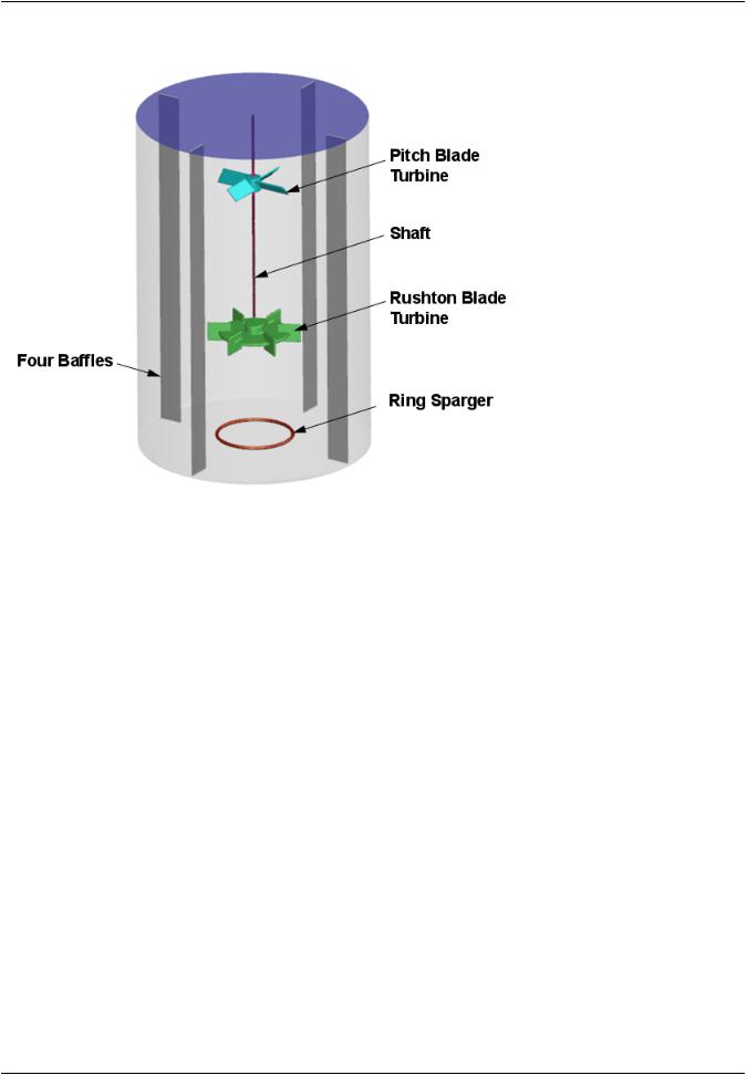
Figure 19.1: Problem Schematic
The geometry consists of a mixing vessel, four baffles along the vessel wall, a ring sparger, a pitch blade turbine, a Rushton blade turbine, and a rotating vertical shaft. There is no water flow into or out of the vessel. Air is injected into the tank at the bottom through the ring sparger at a speed of 0.05 m/s. Small inlet holes in the sparger ring are ignored, and the air inlet is modeled as a uniform circular strip. The air mixes with water, producing small bubbles. The Rushton blade turbine agitates the air-water mixture,
evenly distributing the air bubbles. The pitch blade turbine performs dispersion and pumping operations. Both impellers rotate at 450 rpm in the counterclockwise direction about the Z axis (as viewed from
the top). Dispersed gas bubbles can escape through the top water surface, which is open to the ambient air. This model can be used as a reasonable representation of the initial conditions in a real mixing tank.
19.4. Setup and Solution
The following sections describe the setup and solution steps for this tutorial:
19.4.1.Preparation
19.4.2.Mesh
19.4.3.Solver Settings
19.4.4.Models
19.4.5.Materials
19.4.6.Phases
19.4.7.Cell Zone Conditions
19.4.8.Boundary Conditions
19.4.9.Solution
19.4.10.Postprocessing
19.4.1. Preparation
To prepare for running this tutorial:
|
Release 2019 R1 - © ANSYS,Inc.All rights reserved.- Contains proprietary and confidential information |
658 |
of ANSYS, Inc. and its subsidiaries and affiliates. |

vk.com/club152685050 | vk.com/id446425943 |
Setup and Solution |
1.Download the mixing_tank.zip file here.
2.Unzip mixing_tank.zip to your working directory.
3.The files, mixing_tank.msh, can be found in the folder.
4.Use Fluent Launcher to enable Double Precision and start the 3D version of Fluent. Fluent Launcher displays your Display Options preferences from the previous session.
For more information about the Fluent Launcher, see starting Fluent using the Fluent Launcher in the Fluent Getting Started Guide.
5.Ensure that the Display Mesh After Reading option is enabled.
6.Run in Serial by selecting Serial under Processing Options.
19.4.2. Mesh
1.Read the mesh file mixing_tank.msh.
 File → Read → Mesh...
As Fluent reads the mesh file, it will report the progress in the console.
A warning message will be displayed that the degassing boundary condition type is not compatible with currently enabled models. You will resolve this issue when you enable the Eulerian multiphase model in
asubsequent step.
Click Ok and close the Information dialog box.
2.Check the mesh.
 Domain → Mesh → Check → Perform Mesh Check
Fluent will perform various checks on the mesh and will report the progress in the console. Make sure that the reported minimum volume is a positive number.
3.Display the mesh.
 Domain → Mesh → Display...
a.In the Options group, clear the Faces option and select the Edges option.
b.In the Mesh Display dialog box, select wall_liquid_level, gas-inlet, and Wall (to select all walls) in the Surfaces selection list.
c.Click Display and close the Mesh Display dialog box.
Release 2019 R1 - © ANSYS,Inc.All rights reserved.- Contains proprietary and confidential information |
|
of ANSYS, Inc. and its subsidiaries and affiliates. |
659 |
vk.com/club152685050Using the Multiphase Models| vk.com/id446425943
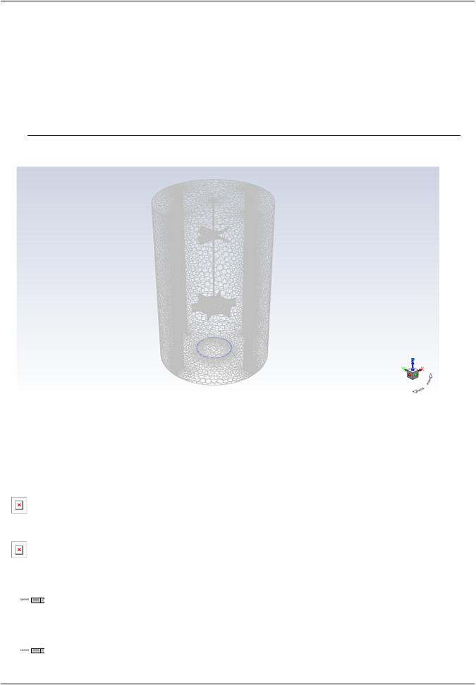
4. Examine the mesh (Figure 19.2: Mesh Display of the Mixing Tank (p. 660)).
Extra
You can use the right mouse button to check which zone number corresponds to each boundary. If you click the right mouse button on one of the boundaries in the graphics window, its zone number, name, and type will be printed in the ANSYS Fluent console. This feature is especially useful when you have several zones of the same type and you want to distinguish between them quickly.
Figure 19.2: Mesh Display of the Mixing Tank
19.4.3. Solver Settings
Related video that demonstrates steps for setting up, solving, and postprocessing the solution results for a two-phase turbulent flow within a mixing tank:
•ANSYS Fluent: Simulating Multiphase Mixing within a Sparging Tank Part I
•ANSYS Fluent: Simulating Multiphase Mixing within a Sparging Tank Part II
1.Retain the default Solver settings.

 Physics → Solver
2.Set the gravitational acceleration.

 Physics → Solver → Operating Conditions...
|
Release 2019 R1 - © ANSYS,Inc.All rights reserved.- Contains proprietary and confidential information |
660 |
of ANSYS, Inc. and its subsidiaries and affiliates. |

vk.com/club152685050 | vk.com/id446425943 |
Setup and Solution |
a.In the Operating Conditions dialog box, enable Gravity to account for gravitational forces.
b.In the Gravitational Acceleration group box, enter -9.81 m/s2 for the Gravitational Acceleration in the Z direction.
c.Select Specified Operating Density.
d.Retain the default value of 1.225 kg/m3 for Operating Density.
For this simulation, you will model air as an incompressible fluid with a density of 1.225 kg/m3, which is a default value.
Note
For multiphase flows, the operating density should be set to the density of the least dense phase.
e.Click OK to close the Operation Conditions dialog box.
f.Click OK to close the Information dialog box.
19.4.4.Models
1.Enable the Eulerian mulptiphase model.
Since you will use the default settings for the Eulerian model, you can enable it directly from the tree by right-clicking the Multiphase node and choosing Eulerian from the context menu.


 Setup → Models → Multiphase
  Eulerian
Click OK to close the Information dialog box.
2.Enable the standard  -
-  turbulence model with standard wall functions.
 Physics → Models → Viscous...
a.Select k-epsilon in the Model group box.
b.Retain Standard in the k-epsilon Model group box.
c.Retain Standard Wall Functions in the Near-Wall Treatment group box.
This problem does not use a particularly fine mesh, and standard wall functions will be used.
d.In the Turbulence Multiphase Model group box, select Dispersed.
The dispersed turbulence model is suitable for cases when the dispersed phase is dilute. The model assumes that turbulence in the primary phase is dominant, while the turbulent quantities of the secondary phase can be obtained from the mean characteristics of the primary phase.
e.Click OK to close the Viscous Model dialog box.
Release 2019 R1 - © ANSYS,Inc.All rights reserved.- Contains proprietary and confidential information |
|
of ANSYS, Inc. and its subsidiaries and affiliates. |
661 |