Chapter 39 Creating a Dynamic Simulation 943

Defining Dynamic Material Properties

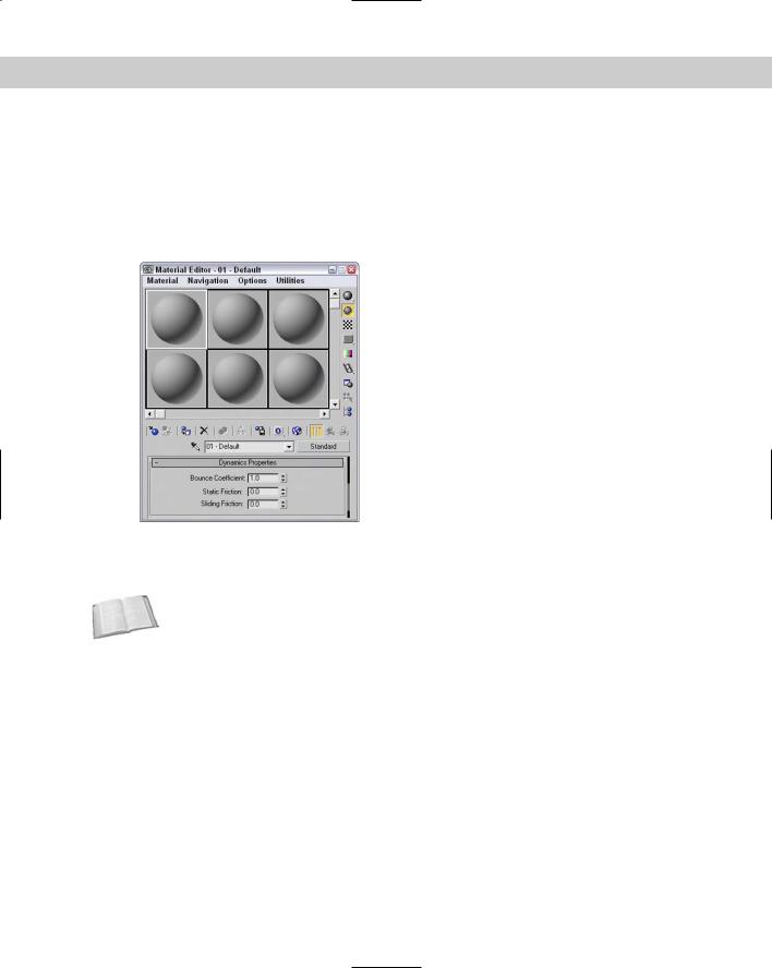
You can use any objects in a dynamic simulation. The Material Editor can endow these objects with materials that include dynamic surface properties. These properties define how the object is animated during collisions in a dynamic simulation and can be accessed in the Material Editor by selecting the Dynamics Properties rollout, shown in Figure 39-4. The default material settings on this rollout are similar to properties for steel.

Figure 39-4: The Dynamics Properties rollout in the Material Editor lets you define physical properties.

Cross-	For more on the Material Editor, see in Chapter 19, “Exploring the Material Editor.”
Reference

The Bounce Coefficient value on the Dynamics Properties rollout determines how high an object bounces after a collision. The default of 1.0 is equal to a normally elastic collision. A ball with a value higher than 1 continues to bounce higher with each impact.

The Static Friction value determines how difficult it is to start an object moving when it’s pushed across a surface. Objects with high Static Friction values require lots of force to move them.

The Sliding Friction value determines how difficult it is to keep an object in motion across a surface. Ice would have a low Sliding Friction value because after it starts moving, it continues easily.

944 Part IX Dynamics

Using Dynamic Space Warps

Several Space Warps are designed to work specifically with dynamic simulations. These can be used to define global effects — such as gravity — that apply to all objects in the simulation.

Space Warps that can be used in a dynamic simulation include all Space Warps in the Particles and Dynamics and the Dynamics Interface subcategories, including Gravity, Wind, Push, Motor, Pin, Bomb, PDynaFlect, SDynaFlect, and UDynaFlect.

Cross-	For details on these Space Warps, see Chapter 38, “Using Space Warps.”
Reference

After you add these Space Warps to a scene, you can specify their binding using the dialog boxes in the Dynamics utility rollouts shown in the next section. You don’t need to bind them with the Bind to Space Warp button.

Using the Dynamics Utility

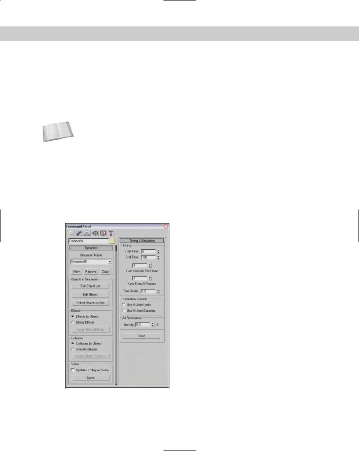
Dynamic simulations are set up and run using the Dynamics utility, which you can find in the Utilities panel. To access the Dynamics utility, open the Utilities panel and click the Dynamics button. Two rollouts open in the Utilities panel, which are shown in Figure 39-5.

Figure 39-5: The Dynamics utility rollouts include buttons for defining which objects to include in a simulation.

Chapter 39 Creating a Dynamic Simulation 945

Using the Dynamics rollout

The Dynamics rollout lets you create a new simulation. To do this, click the New button and enter a name in the Dynamics rollout. You use the Remove button to delete an existing simulation from the list, and use the Copy button to create a new version of the current simulation settings.

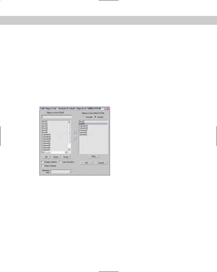
You use the Edit Object List button to add new objects to be included in the simulation. It opens the Edit Object List dialog box, shown in Figure 39-6. This dialog box includes two panes: The one on the left holds all the objects in the scene, and the one on the right holds the objects to include or exclude in the simulation. To include an object in the simulation, select it and click the arrow pointing to the right. This moves the object name to the right pane. Similar versions of this dialog box are used to specify the objects to include in collisions and which effects to include. The Edit Object List dialog box also supports Selection Sets and the Display Subtree, Select Subtree, and Case Sensitive options. After you’ve selected all the objects to include, click the OK button to close the dialog box.

Figure 39-6: The Edit Object List dialog box lets you add objects to the simulation.

You can set object properties for each object included in the simulation. To edit these properties, click the Edit Object button in the Dynamics rollout to open the Edit Object dialog box.

The Select Objects in Sim button in the Dynamics rollout selects the objects in the viewports that are included as part of the simulation, as defined by the Edit Object List dialog box.

You can assign simulation effects in the Edit Object dialog box individually for each object, or you can select the Global Effects option in the Dynamics rollout to make all objects subject to the same effects. The Assign Global Effects button in this rollout opens the Assign Global Effects dialog box (which looks exactly like the Edit Object List dialog box), except that this dialog box lists only the Space Warps included in the scene. Selecting a Space Warp and clicking the right-pointing arrow includes the selected Space Warp as a global effect. Clicking the OK button closes this dialog box.

946 Part IX Dynamics

Collisions are handled in the same way as effects: They can be assigned to react either with specific objects or globally. The Assign Global Collisions button in the Dynamics rollout opens the Assign Global Collisions dialog box (which again looks just like the Edit Object List and Assign Global Effects dialog boxes), where you can select from all the objects included in the simulation. Objects not selected are subject to the other simulation effects but pass right through other objects rather than colliding.

At the bottom of the Dynamics rollout is the Solve button, which creates the actual keys. You can also select the Update Display w/ Solve option to update the viewports as the simulation is solved.

Using the Timing & Simulation rollout

The Timing & Simulation rollout, shown previously in Figure 39-5, specifies the frame range for the dynamic simulation. The Calc Intervals Per Frame value determines how many calculations are made at each frame. This value can range from 1 to 160: The higher the value, the more time is needed to compute the solution.

The Keys Every N Frames setting determines how often keys are created. For example, a value of 2 would create a key for every other frame. You can use the Time Scale to speed or slow a simulation. A setting of 1 is normal speed, values from 0.1 up to 1 slow the animation, and values greater than 1 and up to 100 speed the animation. You can use this setting to create a slow-motion animation of the simulation.

Inverse Kinematics systems can constrain motion through the specification of IK Joint Limits and IK Joint Damping. The Simulation Controls section includes options to enable or disable these settings.

Air resistance is a force that resists motion and is caused by an object crashing into air molecules. Air is denser the closer you are to sea level, which equates to a value of 100. In space, the air density is negligible and is represented by a value of 0.

The Close button at the bottom of the rollout closes the utility.

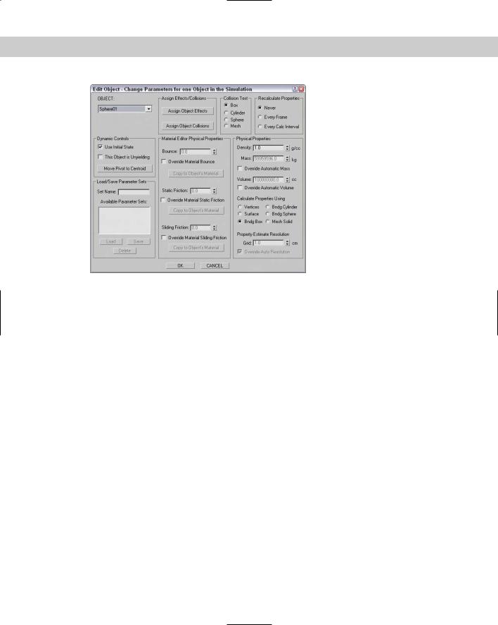
Editing simulation objects

In the Edit Object dialog box, shown in Figure 39-7, you can select which object to edit from the drop-down list in the upper left. This list includes all the objects in the simulation.

In the Dynamic Controls section are two options: Use Initial State and This Object is Unyielding. The Use Initial State option computes the object’s motion and momentum at the start time. If this option is disabled, the object is considered to be motionless at the start time and all existing keys are overwritten during the solution. The This Object is Unyielding option makes sure that the object isn’t moved by collisions during the solution and is the setting to use to simulate a ground plane.

The Move Pivot to Centroid button repositions the object’s pivot to the object’s center of mass. Moving the pivot to the center of mass speeds the simulation calculations, but it alters the positions of any linked objects that are built based on the pivot.

Chapter 39 Creating a Dynamic Simulation 947

Figure 39-7: The Edit Object dialog box lets you assign simulation properties to an object.

In the Load/Save Parameter Sets section, you can save all the parameters in the Edit Object dialog box set by giving the set a name in the Set Name field and clicking the Save button. This parameter set can then be easily loaded and applied to another object. This feature saves you from having to set all the parameters for each object individually. To load a set, select the set from the list and click the Load button.

In the Assign Effects/Collisions section, you can assign each object’s different effects using the Assign Object Effects button. You can also use the Assign Object Collisions button to assign which objects to collide with. These buttons open dialog boxes that are very similar to the Assign Global Effects and Assign Global Collisions dialog boxes.

In the Material Editor Physical Properties section, you can set the same properties for Bounce, Static Friction, and Sliding Friction that can be set for materials in the Material Editor. For each of these, you also have options that enable you to override the setting in the Material Editor as well as copy the property value to the object’s material.

The Collision Test section offers Box, Cylinder, Sphere, and Mesh options for use in computing the collisions between objects. The Box option calculates more quickly than the other options because it uses the object’s bounding box to compute collisions, but these collisions will not be as accurate. The Mesh option determines collisions by looking at the actual object surface, but this option takes the longest to calculate.

The Recalculate Properties section lets you specify how often properties are recalculated. For example, material properties (such as mass) are animatable and can change over the course of an animation — with the volume of an object, for example, increasing as the object is scaled. Recalculation options include Never, Every Frame, and Every Calc Interval. The more often these properties need to be calculated, the longer the calculation takes.

948 Part IX Dynamics

The Physical Properties section enables you to set values for density, mass, and volume. Density is the material thickness of an object, measured in grams per cubic centimeter; mass is the base weight of an object, measured in kilograms; and volume is the space that the object takes up, measured in cubic centimeters. Because these values are interrelated, the Override options enable you to modify them independent of the other values.

The Calculate Properties Using subsection enables you to compute the property values using different volumes, depending on the accuracy you need. Options include Vertices, Surface, Bndg (Bounding) Box, Bndg Cylinder, Bndg Sphere, and Mesh Solid. The bounding options enclose the objects in an easy-to-compute bounding form. The Mesh Solid option increases the computation time significantly. Selecting the Mesh Solid option enables automatic resolution, but you can override this with the Override Auto Resolution option, in which case you can set the Grid value to determine how large each cell in the mesh grid is. These cells are measured in centimeters.

Optimizing a simulation

Solving a dynamic simulation once per frame can generate an enormous number of keys, which can significantly increase the file size. Using the Track View, you can reduce the number of keys while preserving the main keys used in the simulation.

Cross- To learn more about the Track View, check out Chapter 33, “Working with the Track View.”

Reference

After solving a simulation, open the Track View and select the object tracks with keys in them. Then click the Edit Keys button, select all the keys, and click the Reduce Keys button. A simple dialog box opens where you can specify the threshold value.

Tutorial: Bowling a strike

When I go bowling, I get a strike every once in a while, but in Max I can get a strike every time. (I can also secure the pins so that no one can get a strike.)

To run a dynamic simulation of a bowling lane, follow these steps:

1.Open the Bowling set.max file from the Chap 39 directory on the CD-ROM.

This file includes a lane with ten bowling pins and a bowling ball. The lane is surrounded by POmniFlect Space Warps.

Caution	I could have used the plane object for the bowling lane, but the simulation works with the
	actual plane size visible in the viewport. If the simulation were solved, a warning would appear
	stating that the plane object has unshared edges, and the results could be unpredictable.

2.Select the Create Space Warps Forces Gravity menu command, and drag in the Front viewport to create a Gravity Space Warp. Position this Space Warp behind the bowling ball, and point it at the bowling ball to give some thrust to the ball. In the Parameters rollout, set the Strength to 10.

3.Open the Utilities panel, and click the Dynamics button to open the Dynamics rollout. Click the New button to create a new simulation. Then click the Edit Object List button, select all the objects in the left pane, move them to the right pane by clicking the arrow pointing to the right, and click OK.

Chapter 39 Creating a Dynamic Simulation 949

4.Select the Effects by Object option in the Effects section of the rollout. Click the Edit Object button, and select the Bowling ball object in the Object drop-down list in the upper-left corner. Then click the Assign Object Effects button, double-click the Gravity Space Warp to move it to the right pane, and click OK. Next select the Lane object, enable the This Object is Unyielding option, and click OK.

Note Because Space Warps are assigned using the Dynamics rollout, you don’t need to use the Bind to Space Warp button.

5.In the Collisions section of the Dynamics rollout, select the Global Collisions option and click the Assign Global Collisions button. Click the All button to select all the objects in the left pane, and move them to the right pane by clicking the arrow pointing to the right. Then click OK.

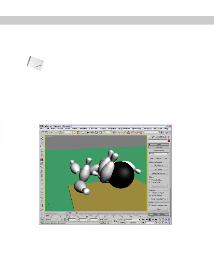
6.In the Timing & Simulation rollout, set End Time to 40. Then select Update Display w/ Solve, and click the Solve button. The simulation frames display in the viewport. After the solution is finished, click the Play Animation button to see the entire simulation.

Figure 39-8 shows a frame of the resulting simulation. Keep in mind that only the collision and simple gravity are in effect, but in reality many other forces exist. The final animation for this example shows the pins being blasted off into space.

Figure 39-8: This simulation of a bowling game computed all the collisions between the bowling pins and the bowling ball.